4.5 Normal Distribution

4.5: Normal Distribution
Learning Objectives
Upon completion of this section, you should be able to
- Describe features of a normal distributions
- Use the Empirical Rule (68-95-99.7 Rule) with applications involving the normal distribution
- Find z-scores for values based on a normal distribution
- Find a percentile for a given z-score using the standard normal table
- Solve applied problems involving normal distributions and the standard normal table
Normal Distribution
One of the things we have looked at in the descriptive statistics sections is a way to describe a particular set of data, whether it be quantitative or categorical (qualitative). A next step we can take is to classify what type of distribution the data may have come from (this allows us to answer very interesting questions about the population). We will focus our time on this concept by looking at a very common distribution named the Normal Distribution. The normal distribution is recognized with its characteristic bell shape, but not all bell shaped distributions must be a normal distribution. The distribution itself only needs the mean and standard deviation to completely describe its shape and properties.
Normal Distribution
The normal distribution is a symmetric distribution in a shape of a bell (sometimes called the bell curve). It is described by the parameters of the mean μ and standard deviation σ. The graph below shows how the bell shape and parameter values identify key portions of the graph on how the bell turn at key points for the shape. The peak of the bell occurs at the mean for the distribution and the graph turns in concavity one standard deviation away from the mean in both directions.
The Normal Distribution plays an important role in many inference procedures in Statistics. We will study some of the properties of the Normal Distribution to give you an idea of what we can say once we are able to identify clearly what the distribution of a variable is from a population. Just keep in mind just because a graph looks bell shape doesn’t necessarily mean it will be in general a normal distribution that describes the data.
Strictly speaking, it is not correct to talk about “the normal distribution” since there are many normal distributions. Normal distributions can differ in their means and in their standard deviations. Figure 1 shows three normal distributions. The green (left-most) distribution has a mean of -3 and a standard deviation of 0.5, the distribution in red (the middle distribution) has a mean of 0 and a standard deviation of 1, and the distribution in black (right-most) has a mean of 2 and a standard deviation of 3. These as well as all other normal distributions are symmetric with relatively more values at the center of the distribution and relatively few in the tails.
Some features of normal distributions are listed below.
- Normal distributions are symmetric around their mean.
- The mean, median, and mode of a normal distribution are equal.
- Normal distributions are denser in the center and less dense in the tails.
- Normal distributions are defined by two parameters, the mean (μ) and the standard deviation (σ).
- 68% of the area of a normal distribution is within one standard deviation of the mean.
- Approximately 95% of the area of a normal distribution is within two standard deviations of the mean.
- Approximately 99.7% of the area of a normal distribution is within three standard deviations of the mean.
Each different choice of specific numerical values for the pair μ and σ gives a different bell shaped curve. The value of μ determines the location of the center for the curve, as shown in Figure 2 “Bell Curves with different values of μ”. In each case the curve is symmetric about µ.
In figure 2 the standard deviation was the same for each normal distribution, but only the mean was changed. What we see is that the mean determines where the center of the distribution is, but doesn’t change with width or spread of the distribution. Visually it appears the distribution is just a copy of each other shifted left or right depending on the value of the mean.
The value of σ determines whether the bell curve is tall and thin or short and squat, subject always to the condition that the total area under the curve be equal to 1. This is shown in Figure 3 “Bell Curves with different values of σ”, where we have arbitrarily chosen to center the curves at μ = 6.
We just spent some time going over the shape of a normal distribution. Let’s put some of these ideas together with an example of a population that has a normal distribution to see what we can say about the population just by knowing it is normal with a given mean. In the next topic for this page we will explore further how we can answer questions about the population by knowing it follows a normal distribution.
Example 1
Heights of 25-year-old men in a certain region have mean 69.75 inches and standard deviation 2.59 inches. These heights are approximately normally distributed.
- Construct a rough sketch of the normal distribution labeling the mean and one standard deviation from the mean on the horizontal axis.
- What percent of men have a height above 69.75 inches?
Solution
- The graph of the normal distribution is displayed below.
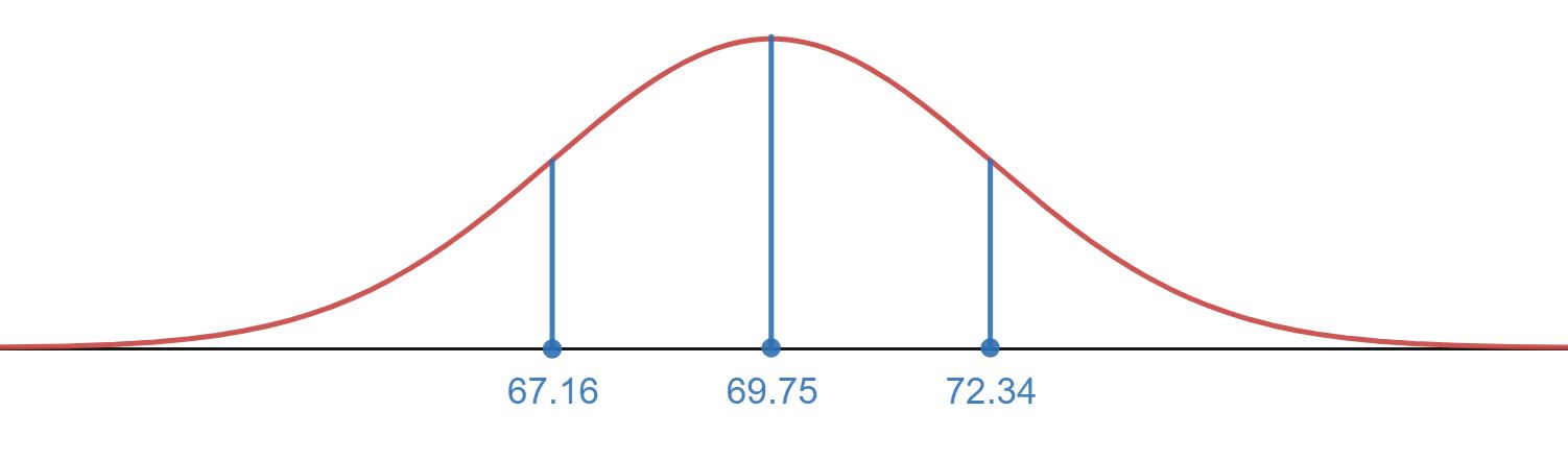
- The normal distribution is symmetric about the mean. This means 50% of the population would be above the mean and 50% of the population would be below the mean. We can conclude 50% of men have a height above 69.75 inches.
Empirical Rule (68 – 95 – 99.7 Rule)
Below is a rough sketch of a Normal Distribution along with what we know about the amount of data within 1, 2, or 3 standard deviations about the mean. On the graph the peak is where the mean is (which would also be the median and mode value for the data set). These Rules apply to most Bell Shaped curves (there are some exceptions, but for the ones you will see in this course you may assume the rule applies).
Empirical Rule (68 – 95 – 99.7 Rule)
The empirical rule or the 68 – 95 – 99.7 Rule states that for a normal distribution we are able to determine the area under the curve in regions one, two, or three standard deviations from the mean.
- About 68% of all values fall within 1 standard deviation of the mean.
- About 95% of all values fall within 2 standard deviations of the mean.
- About 99.7% of all values fall within 3 standard deviations of the mean.
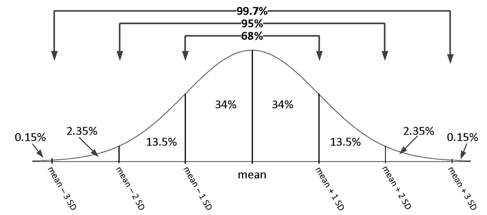
It is helpful for any problem you work on to start with a general visual for the normal distribution and then label the values of the mean and standard deviation values to help answer questions in the application. The image below is the baseline for drawing that normal distribution as it includes 1, 2, and 3 standard deviation values below and above the mean. The areas then for each region can be taken from the image above.
Example 2
Suppose we have a normal distribution with a mean of 10 and standard deviation of 2.
- What is the percentage of the population that has a value between 8 and 12?
- What is the percentage of the population that has a value below 12?
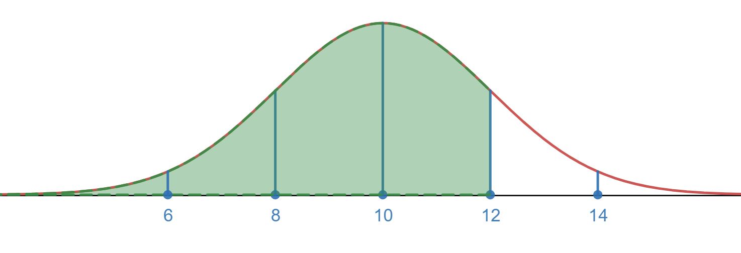
- What is the percentage of the population with values between 6 and 12?
Solution
- To use the empircal rule it is best to visualize the distribution along with the region we are looking for.
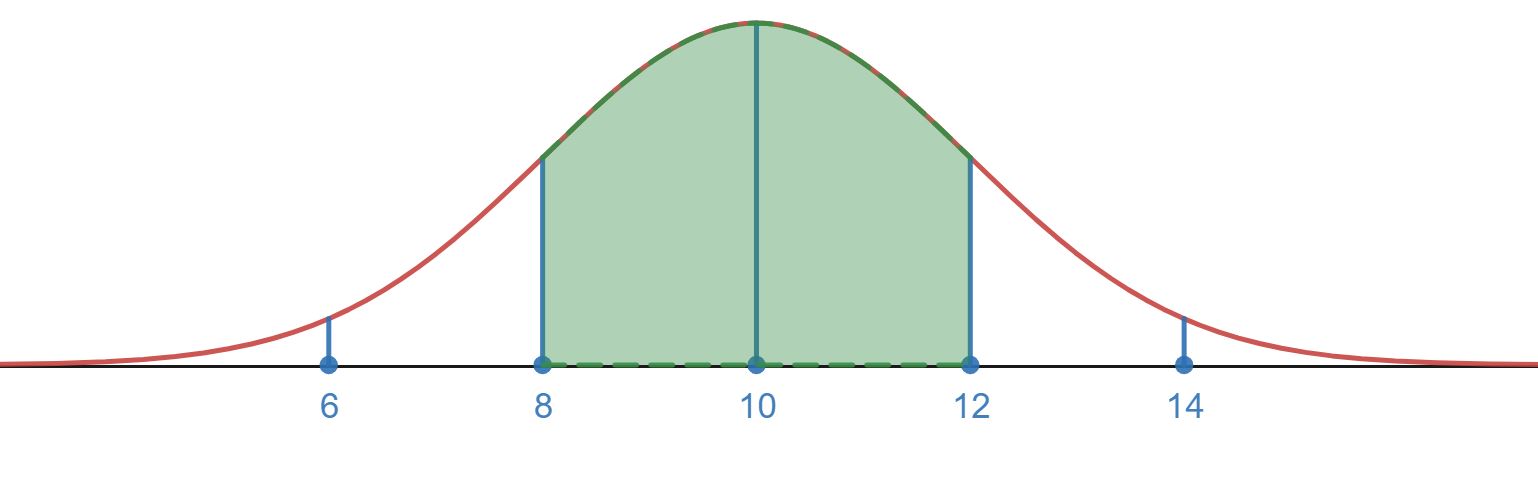
The value 8 is one standard deviation below the mean, since 10-2=8. The value 12 is one standard deviation above the mean, since 10+2=12. By the empirical Rule we have 68% of the population is between 8 and 12.
- Visualize the region of interest before jumping into a strategy to solve the problem.
Break the total region into two parts. We have one part that is everything below the mean and the other part between 10 and 12 that is one standard deviation above the mean. We can use the fact that the normal distribution is symmetric about the mean along with the the empirical rule to find the percent of the population below 12. We know two things from this fact and the empirical rule:
- 50% of the population is below the mean (normal distribution is symmetric about the mean).
- 68% of the population is between 1 standard deviation above and below the mean (empirical Rule)
Since 68% is the percentage between 1 standard deviation above and below the mean we can say that is the percentage above the mean to 1 standard deviation away (this would be the interval from 10 to 12).
Now add to that the 50% below the mean (this would be the interval for everything below 10) we have that 84% of the values are below 12 or 1 standard deviation above the mean.
- The visual for the interval from 6 to 12 is shown below.
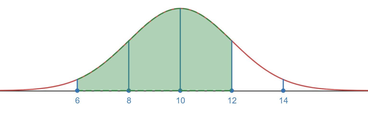
Using the information from b. we know that from 10 to 12 (the mean to one standard deviation above the mean) we have 34% of the values. The empirical Rule and symmetry argument like in b. will help us figure out what percentage goes from 6 to 10.
We can see 6 is 2 standard deviations below the mean (6=10-2*2). The empirical Rule tells us that about 95% of the values are between two standard deviations above and below the mean, so this means 95% of the observations are between the values 6 and 14. We can use the symmetry of the normal distribution to say that must mean only of the values occur between 6 and 10 (between the mean and two standard deviations below the mean).
Putting this together we see that there is a total of 34%+47.5%=81.5% of the values between 6 and 12.
Example 3
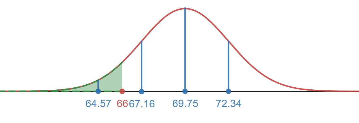
Heights of 25-year-old men in a certain region have mean 69.75 inches and standard deviation 2.59 inches. These heights are approximately normally distributed. Answer the following questions using the Empirical Rule. If the rule does not apply state why.
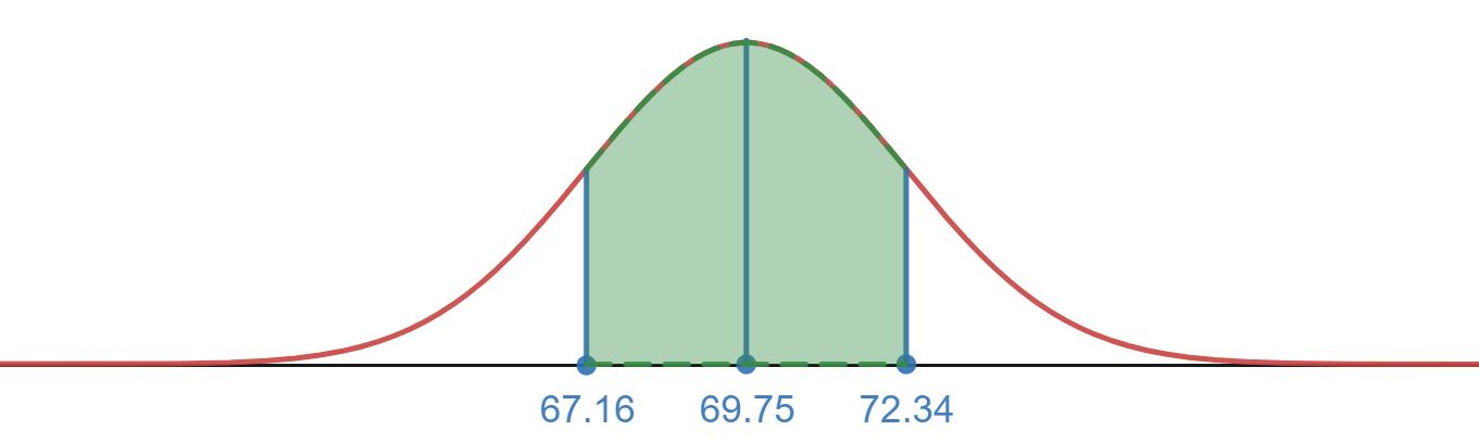
- What percent of men have a height between 67.16 and 72.34 inches?
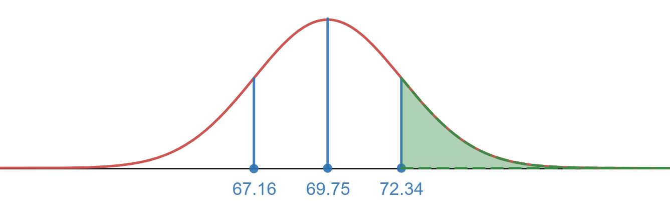
- What percent of men have a height above 72.34 inches?
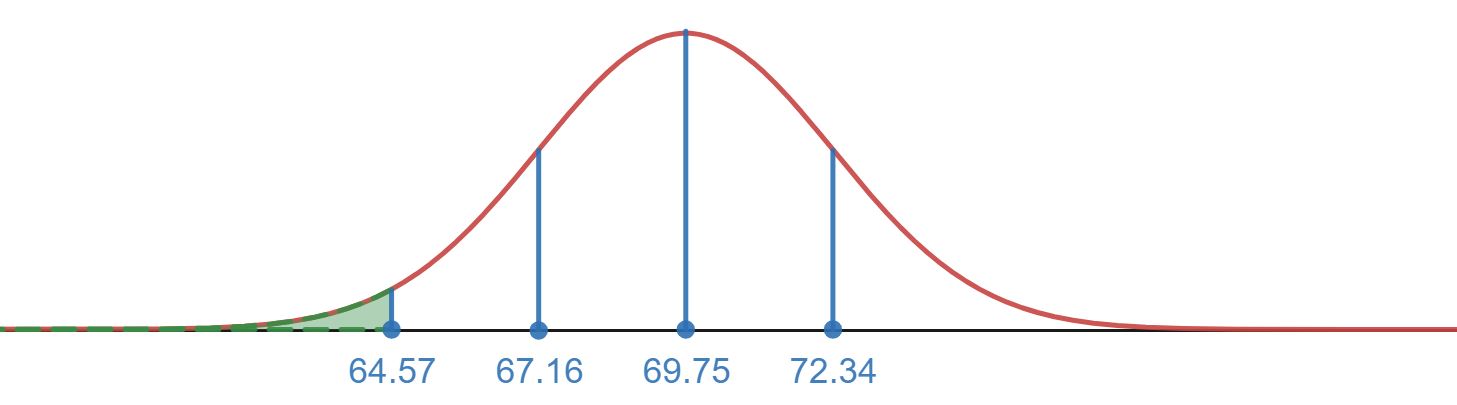
- What percent of men have a height below 64.57 inches?
- What percent of men have a height below 66.0 inches?
Solution
As you go about answering these draw a shaded in diagram of a normal distribution to represent the area of interest to help guide you in your work.
- The region shown below illustrates the shaded in region for one standard deviation above and below the mean. From the empirical rule we know this region represents 68% of the population.
- The region shown below that is shaded in shows we are looking at everything one standard deviation above the mean. The empirical rule can help us find this area along with knowing 50% of the population would be above the mean. From the empirical rule we know the region from 69.75 to 72.34 would have 34% percent of the population (this is half of the 68% from one standard deviation above and below the mean). Since 50% is above the mean we can subtract the 34% away to find the remaining upper tail shaded in below:
- The region shown below that is shaded in shows we are looking at everything two standard deviations and below the mean. We can use a similar strategy as part b above. We know 50% of the population would be below the mean and the empirical rule tells us that would be two standard deviations below the mean. This means the percent below 64.57 would be
- The shaded in region below 66 is shown below. The empirical rule only gives us tools to find the percentage of a population that falls at 1, 2, or 3 standard deviations away from the mean. The value 66 appears to fall between 1 and 2 standard deviation below the mean, so we cannot use the empirical rule to find this percent of the population.
The video below is from Sal at KhanAcademy. Please remember to pause the video and attempt the problem on your own (you may need to listen to the details as the text is hard to read).
Normal distribution problems: Empirical rule | Probability and Statistics | Khan Academy
(10 mins 25 secs – CC).
Now it is your turn to practice with the Empirical Rule.
Try it Now 1
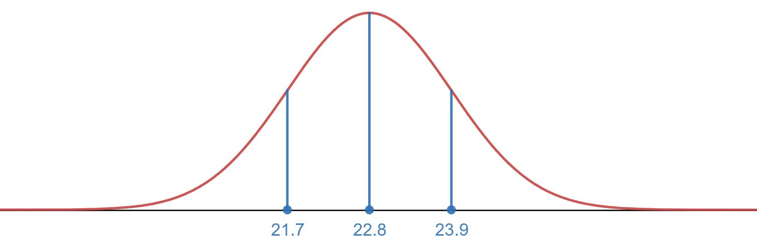
It is known that the head circumference among soldiers has a mean of 22.8 inches and a standard deviation of 1.1 inches. It is also known that the distribution has a bell shaped curve to it (i.e. a Normal Distribution).
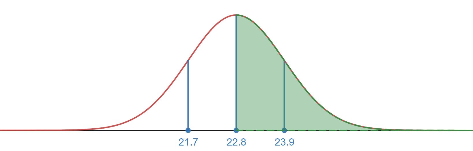
- What % of soldiers heads have a circumference larger than 22.8?
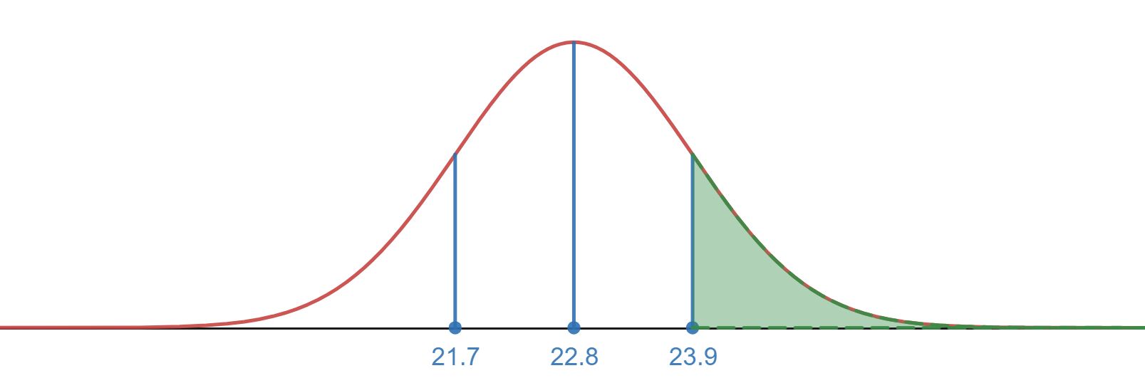
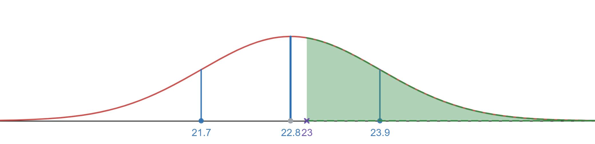
- Larger than 23.9?
Hint 1 (click to Show/Hide)
The graph of the normal distribution shows us half of the region is above the mean and the other half is below. This should make answering the first part a bit easier. For the second part you may want to draw the normal distribution and see if there is a way to use the empirical rule to find the percentage above 23.9
Below is the graph of the normal distribution to help you shade in the region of interest for each part.
Answer (click to Show/Hide)
- 50%, since a normal distribution is symmetric about the mean.
- 16%, We know by the empirical Rule and symmetry that 34% of the head circumferences fall between 22.8 and 23.9 inches (68% of the empirical Rule and Symmetry). By symmetry we also know that 50% are smaller than 22.8 inches. This gives us a total of 84% of head circumferences that are smaller than 23.9 inches. The remaining 16% must then be larger than 23.9 inches.
Z-Scores
Can we still determine percentages of observations for a normal distribution if we are not 1, 2, or 3 standard deviations away from a mean (i.e. can we find the area under a normal distribution where the starting or ending points are not 1, 2, or 3 standard deviations away from the mean)? The answer is yes, but the methods for doing so will vary depending on what tools you have available to you. The method we will use below uses the idea of still measuring how many standard deviations away from the mean an observed data value is. That signed distance is what we will call a z-score.
Z-score
A z-score represents the number of standard deviations that a given value in a data set (or distribution) is above or below the mean. We calculate a z-score by using the following formula:
- x is the data value we’re interested in
- μ (mu) is the mean of the dataset
- σ (sigma) is the standard deviation of the dataset
A positive z-score means the data value is above the mean, while a negative z-score indicates it’s below the mean. A z-score of 0 means the value is exactly at the mean.
Example 4
Heights of 25-year-old men in a certain region have mean 69.75 inches and standard deviation 2.59 inches. These heights are approximately normally distributed. Find the z-score for a height of 66.0 inches. Round to the nearest hundredth.
Solution
Based on our work from Example 2 we saw that 66.0 was below the mean, so we expect to have a z-score that is negative:
The z-score is approximately -1.45. Negative as we expected as 66 is 1.45 standard deviations below the mean of 69.75.
One of the things we can use z-scores for is to compare two data points from different normal distributions. What the z-score tells us is how far away the data point is from the mean of the population it is from. The further away the more extreme that data value is.
Example 5
Brand A tire has a mean life of 45,000 miles and a standard deviation of 4,500 miles. Brand B has a mean life of 38,000 miles and a standard deviation of 2080 miles. Suppose somebody with a Brand A tire lasts 48,000 miles while someone with Brand B tire lasts 40,000 miles. Which driver got a better deal from their tire?
Solution
We do notice that they both had better mileage than the mean (Brand A was 3,000 miles above the mean and Brand B was 2,000 miles above the mean). Brand A had more mileage above the mean, but does it mean it was better relative to the tires in its own population? The answer to this would depend on how far from the mean it was in a relative distance to the population’s measure of spread (the standard deviation). The z-score will tell us that distance from the mean in terms of the standard deviation – we can use this to compare to the Brand B tire.
The Brand B tire was further from the mean based upon the calculated z-score (remember this calculation includes the relative size of the dispersion of the population). The person with the Brand B tire received better performance out of all Brand B tires in the population than the Brand A owner did in the Brand A population. The Brand B driver got a better deal in terms of performance of the tire in the population of Brand B tires as fewer Brand B tires would have lasted longer when compared to the Brand A tire.
Try it Now 2
At a particular school there was concern about grade inflation. One solution presented was to issue standardized grades in addition to the regular course grade for students’ records. For each class a student received a score (from 0 to 4) and the class mean and standard deviation of scores were recorded.
For a given student Camila the scores for four classes were recorded. If we were to judge by standardized grades which class did Camila do best in? Which course did she do the worst?
| Camila’s Score | Mean for Class | Standard Deviation for Class | |
|---|---|---|---|
| WRT 101 | 3.55 | 3.15 | .30 |
| MAT 142 | 3.60 | 3.05 | .45 |
| BIO 201IN | 3.40 | 2.95 | .50 |
| PSY101 | 3.55 | 3.65 | .15 |
Hint 1 (click to Show/Hide)
For each class calculate the z-score and then compare to see which score was the highest (that will be class she did the best in) and which score was the lowest (that would be the class she did the worst in).
Answer (click to Show/Hide)
| Course | Z-score |
|---|---|
| WRT 101 | |
| MAT 142 | |
| BIO 201IN | |
| PSY101 |
The highest z-score was in WRT 101, so Camila did best in that course. The lowest z-score was from PSY 101, so in that class she did the worst. The interesting thing to point out is that in both WRT 101 and PSY 101 she received the same score, so when dealing with different populations (classes) we cannot directly compare data values to each other.
Z-Score Percentiles
The idea of using a z-score was sort of introduced to solve problems relating to percentages of a normal distribution through the use of the empirical Rule (think about it – we were looking at being 1, 2, 3 for the value of a z-score in those problems). What do we do if the regions of interest on that normal distribution are not exactly 0, 1, 2 or 3 standard deviations away? We can’t use our empirical rule to solve that problem and will have to rely on another method. One way to approach these types of problems is to relate the region of interest to an equivalent region of interest on the standard normal distribution. We can do this by converting key values to a z-score.
How does converting a value to a z-score help us?
If the data values come from a normal distribution, then these z-scores will also be a normal distribution, but this normal distribution is guaranteed to have a mean, μ, of 0 and a standard deviation, σ, of 1. We call this the Standard Normal Distribution.
Standard Normal Distribution
A standard normal distribution is a normal distribution with mean μ = 0 and standard deviation σ = 1. It will always be denoted by the letter Z.
The way to calculate the percentage below a given z-score can be found by using a table of values from a standard normal distribution (depending on where the table comes from there are different ways to read these – we will use the table provided in the link for our calculations). Print out the pdf version for your own reference as you go through these problems.
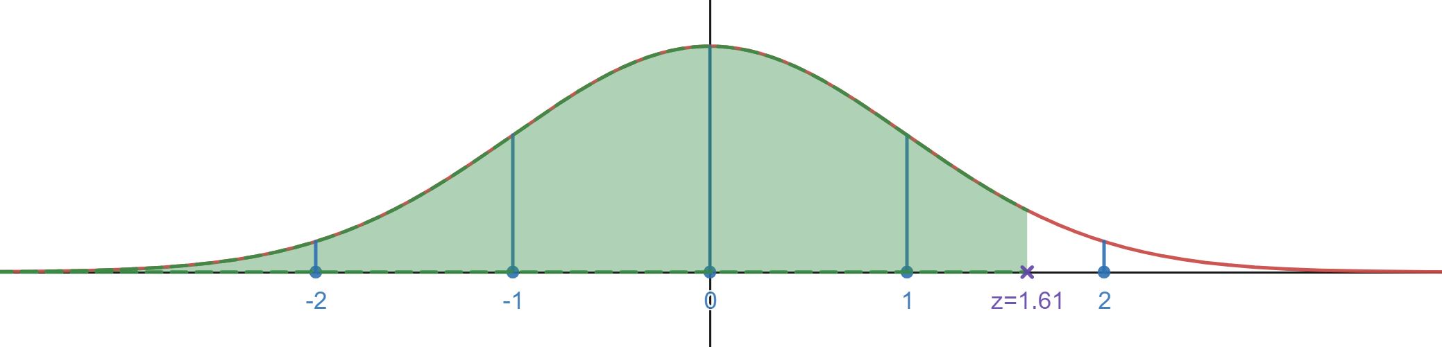
We use the table by breaking up the z-score into two parts and finding a corresponding row and column that represents that number. To break up the z-score we rewrite the number to the tenth place and then keep track of the hundredth digit. For instance z = 1.61 is broken into z = 1.6 and 0.01. On the table we go down until we see 1.6 in the first column. Next we go to the right to match the column with .01. The value at the intersection of row 1.6 and column 0.01 is then recorded, so in this case 0.9463.
The value 0.9463 is the percentile for z = 1.61. That percentile represents the percentage of the population that had a z-score below your given value. For instance z = 1.61 tells us that 94.63% of the population has a z-score lower than 1.61. Remember the z-score is interpreted as how many standard deviation for the mean the data point was, so z = 1.61 says that the data value is 1.61 standard deviations above the mean. The graph below gives a visual of the z-score value z = 1.61 and the percentile region as shaded in for a standard normal distribution.
Percentile
Given an observed value x in a data set, x is the P th percentile of the data if the percentage of the data that are less than or equal to x is P.
This percentile value will also be referred to as the area under the curve to the left of the given z-score on a standard normal distribution.
Example 6
Find the percentiles for the indicated z-score.
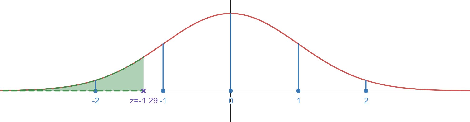
- z = -1.29
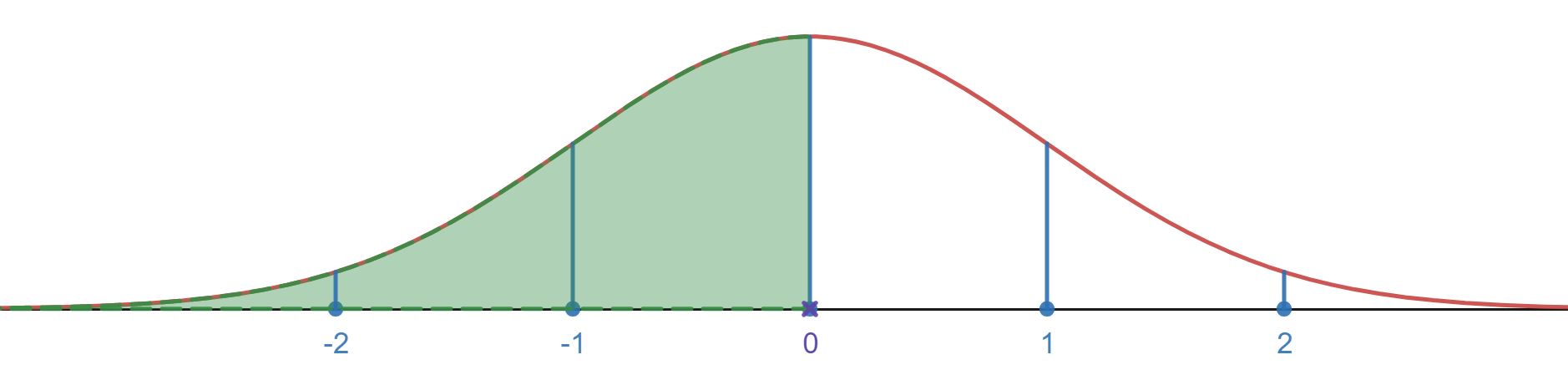
- z = 0
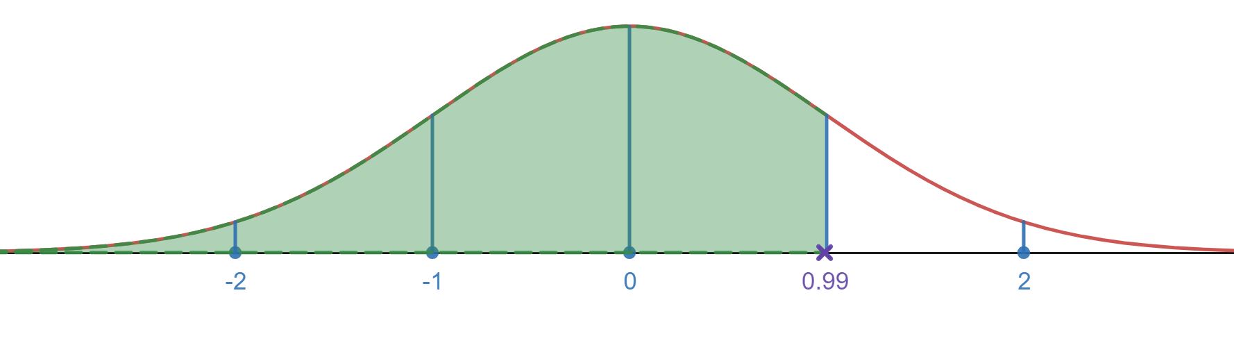
- z = 0.99
Solution
- Using the z-score table we find the percentile for z = -1.29 as 0.0985 or 9.85%
- Using the z-score table we find the percentile for z = 0 as 0.5000 or 50.00%
- Using the z-score table we find the percentile for z = 0.99 as .8389 or 83.89%
In the next example we will find the percentage of values for various regions on the standard normal distribution.
Example 7
Find the percentage of values for each interval given below:
- 0.5 < z < 1.57
- -2.55 < z < 0.09
Solution
-
The z-score table already gives the percentage of values below a given z-score (also known as the area under the curve up to a given z-score). From the table for we read that the percentage (or area) is .9306 for .
Shaded in region under Standard Normal Distribution that represents the percentage of value for z < 1.48. 
-
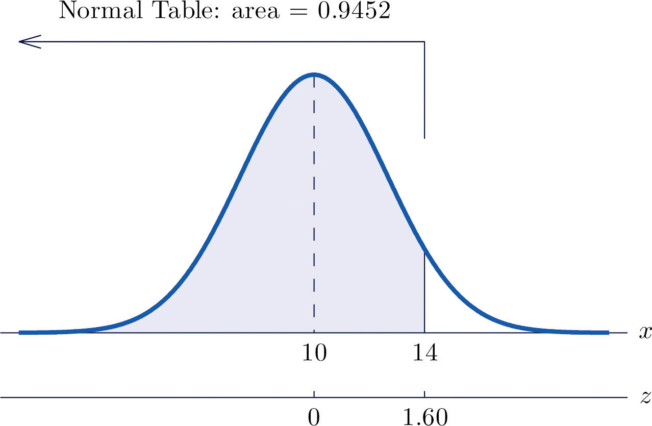
To find the percentage above 1.60 we are going to run into a problem by just trying to pull the value off directly on the table. The table only gives area to the left, so visually we are not getting the correct value directly. Since the total area under the curve is equal to 1 if we have the area to the left we can subtract that from 1 to find the area to the right for .
The table gives a value for as 0.9452, so the percentage above will be .
Shaded in region under Standard Normal Distribution that represents the percentage of value for . 
-
To find the percentage of values between first look up the areas in the table that correspond to the numbers 0.5 (which we think of as 0.50 to use the table) and 1.57. We obtain 0.6915 and 0.9418, respectively. The value 0.9418 represents the percentage shaded in below , but we do not want all of that area. Take away from 0.9418 what we don’t want, which is the shaded in area below . The table gave us the value 0.6915 for that area. The difference of these two numbers give the percentage desired: .
Shaded in region under Standard Normal Distribution that represents the percentage of value for z between 0.5 and 1.57 
-
Using a similar strategy as c and subtract the percentiles found from the table from both z-scores. The percentage between -2.55 and 0.09 is: .
Shaded in region under Standard Normal Distribution that represents the percentage of value for z between 0.09 and -2.55 
Normal Distribution Applications
Now we are ready to tackle problems related to a normal distribution. We will be looking at how to find the percentage of values that will fall within certain regions of a normal distribution. The way we can answer the questions is to identify the region of interest on a normal distribution curve. Identify any key points (start and end points for the intervals of interest). Convert those key points to z-scores and use the standard normal table to find the percentiles. From there we construct an equation (if needed) to find the percentage related to our interval of interest.
In the examples that follow it is helpful to always draw the normal distribution and shade in the region of interest. This will help decide what to do with values from the standard normal table. Try not to skip the step of drawing the normal distribution as work on the additional exercises below the examples.
Example 8
A normal distribution has a mean of 10 and a standard deviation of 2.5. Find the percentage of values below 14.
Solution
Start with identifying the region of interest on the normal distribution. We want to find the percentage of values that fall below the value of 14. Draw the normal distribution and label the mean. Label 14 (the key point here as we want the percentage below 14).
Find the z-score:
The percentile that corresponds to a z-score of 1.60 on the table is 0.9452, so this means 94.52% of the values on this normal distribution are below a value of 14.
Let us revisit the example of male heights and use the standard normal table to help us solve the question from example 2.
Example 9
Heights of 25-year-old men in a certain region have mean 69.75 inches and standard deviation 2.59 inches. These heights are approximately normally distributed. Find the percentage of men whose heights are below 66.0 inches.
Solution
Start with drawing the normal distribution as we did earlier in example 2 and show the shaded region we are interested in.
To find this percentage we will convert the 66.0 to a z-score. Next we will go to the standard normal table and pull out the percentage of the population that fall below the z-score. That value will give us the percent we are interested in since it corresponds to the area to the left under the normal curve. If you were looking for the percentage above we would need to take one additional step of subtracting the value from 100%.
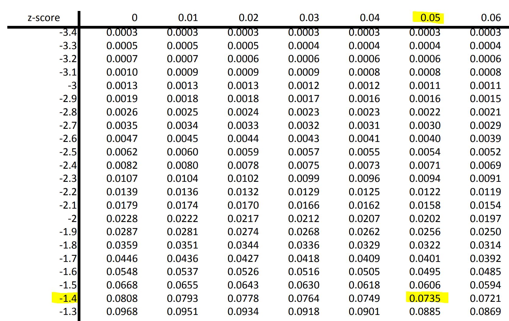
With a z-score of -1.45 we go to the standard normal table and see the corresponding value is .0735 which means 7.35% of the population is below that given z-score of -1.45. We can conclude then that 7.35% of men (from the given region) have a height below 66.0 inches.
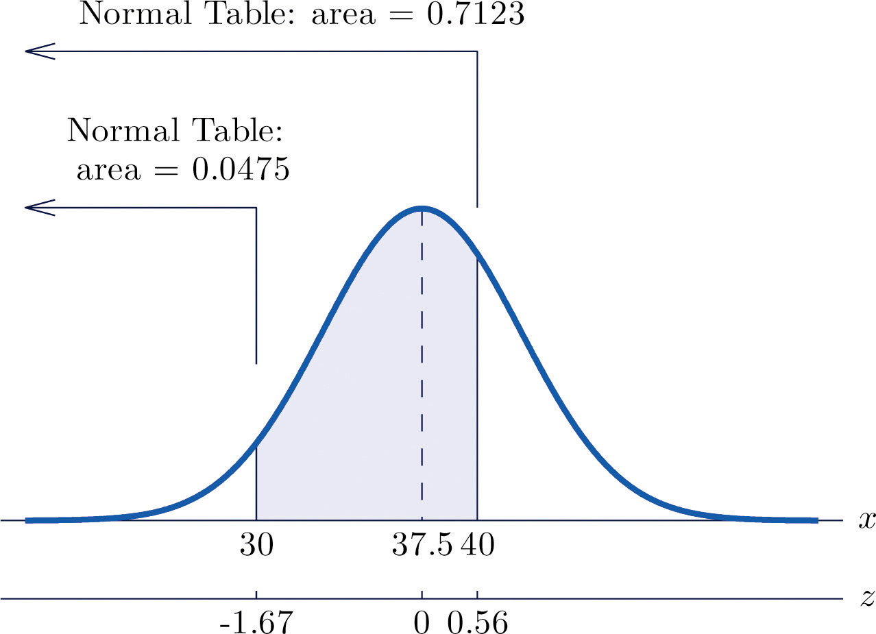
Example 10
The lifetimes of the tread of a certain automobile tire are normally distributed with mean 37,500 miles and standard deviation 4,500 miles. What percentage of tread lives will be between 30,000 and 40,000 miles?
Solution
We are looking for the percentage between two values under the number distribution. Convert each endpoint to a z-score and use the standard normal table to find the percentage of values below that given z-score. The difference between those two percentiles will be the percentage of values between them.
Find the z-score for 30,000:
Find the z-score for 40,000:
The standard normal table reads 4.75% of all values fall below the z-score of -1.67. For z-score of 0.56 we have 71.23% of all values falling below it. As illustrated below the area between them is going to be the difference of these two values: .
Try it Now 3
It is known that the head circumference among soldiers has a mean of 22.8 inches and a standard deviation of 1.1 inches. It is also known that the distribution has a bell shaped curve to it (i.e. a Normal Distribution).
- What % of soldier heads have a circumference larger than 23 inches?
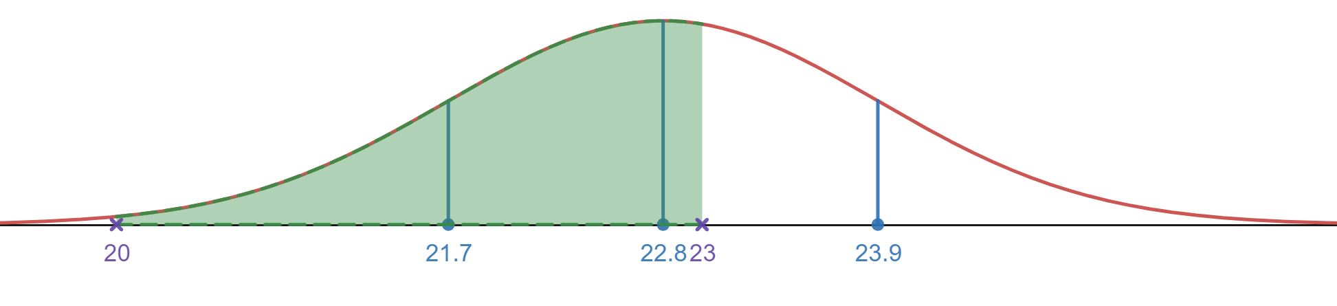
- Between 20 inches and 23 inches?
Hint 1 (click to Show/Hide)
If you want to use the empirical rule you have to check to see if the points of interest are exactly one, two, or three standard deviations away. The mean is 22.8 with a standard deviation of 1.1. The point of interest is 23, which is not one standard deviation above, but lower than one standard deviation above. To answer this question you will need to find the z-scores so that you are able to use the z-table to find percentages. The table won’t directly answer the questions, but you can use it to build up the answer with a little work.
Hint 2 (click to Show/Hide)
-
Shaded in area for the interval above 23 inches on the normal distribution.
-
Shaded in area for the interval between 20 and 23 inches on the normal distribution.
Answer (click to Show/Hide)
-
Shaded in area for the interval above 23 inches on the normal distribution.
First calculate the z-score for 23 inches and then use the table to find the percentage below that given z-score:
Now we have we will round this to to use the table to find the percentage of soldiers whose head circumference is “below” 23 (remember that values in the table are for the percentage below a number – we will need to subtract this from 100% to find the percentage above 23 inches).
Using we have from the table a result of 57.14% or in terms of the application 57.14% have a head circumference below 23 inches. This means have a head circumference larger than 23 inches.
-
Shaded in area for the interval between 20 and 23 inches on the normal distribution. It may be hard to see that region below 20 is not shaded.
First find the z-scores and resulting percentages for the values 20 inches and 23 inches (we already have from above that 57.14% have a head circumference below 23 inches).
Using we know from the table that 0.54% have a head circumference below 20 inches.
To find the percentage beteween 23 and 20 we will take the total percent below 23 and subtract off the region below 20 that we just found:
We have 56.6% of the soldiers with a head circumference between 20 and 23 inches.
Exercises
- The normal distribution is defined by two parameters. What are they?
Answer (click to Show/Hide)
The mean μ and standard deviation σ.
- True/false: For any normal distribution, the mean and median will have the same value.
Answer (click to Show/Hide)
True. The distribution is symmetric about the mean, so the middle value and most frequent would also be at that location of the mean.
- True/false: The proportion of values above the mean is 50%.
Answer (click to Show/Hide)
True. The normal distribution is symmetric about the mean. This means 50% of the values is above the mean and 50% of the values are below the mean.
- True/false: A normal distribution has a mean of 60 and a standard deviation of 10. 68% of the values fall within 60 to 70.
Answer (click to Show/Hide)
False. That region would be 34% as it represents just the first half used in the empirical rule for one standard deivation below and above the mean being 68% of the data values.
- True/false: A normal distribution has a mean of 60 and a standard deviation of 10. You can use the empirical rule to find the percent of values between 55 and 65.
Answer (click to Show/Hide)
False. The value 55 is .5 standard deviations away from the mean, so we can’t use the empirical rule to find a percentage of values based on the value of 55.
- A normal distribution has a mean of 80 and a standard deviation of 12. What values are within one standard deviation of the mean?
Answer (click to Show/Hide)
68 and 92 are both one standard deviation from the mean, so any values between 68 and 92 are within one standard deviation of the mean.
-
- What proportion of a normal distribution is within one standard deviation of the mean?
- What proportion is more than 2.0 standard deviations from the mean?
Answer (click to Show/Hide)
- 68%. The 68-95-99.7 rule tells us that 68% of the data values are within one standard deviation of the mean if the distribution is a normal.
- 95%. For part “b” using the same rule we know 95% of the data values are within 2 standard deviations from the mean, which leaves us 5% in the tales of that bell shaped curve. Since the Normal distribution is symmetric about the mean the tails must share that 5% evenly and leaves 2.5% above two standard deviations above the mean.
- What proportion of a normal distribution is above one standard deviation from the mean?
Answer (click to Show/Hide)
16%, we know that 68% of the data is between one standard deviation below and above the mean. This means the region below one standard deviation below the mean and the region above one standard deviation above the mean share a total of 32% of the remaining area. Due to the symmetry about the mean both of these have the same area, so the total area above one standard deviation above the mean is half of that value which is 16%.
- A company that makes frozen pizzas knows that the pizza that are made have a diameter with a mean of 9.2 inches with a standard deviation of .1 inch. They advertise the pizzas as 9 inch pizzas. Use the empirical Rule to determine what percentage of pizzas made are actually smaller than 9 inches.
Answer (click to Show/Hide)
2.5%. The 68-95-99.7 rule tells us that 95% of the data values are within two standard deviation of the mean if the distribution is normal. With a mean of 20 and a standard deviation of 4 we know two standard deviations from the mean is between the values 12 and 28. We are interested in the percent of values below 12. The 95% tells us that there must be 5% in the tales of that bell shaped curve. Since the Normal distribution is symmetric about the mean the tails must share that 5% evenly and leaves 2.5% in the tale on the distribution that represents the values below 12.
- The exam scores for a large class is approximated by a normal distribution with a mean of 72 and standard deviation of 8. Answer the following questions using the empirical Rule, if it is not possible to use the empirical Rule state why.
- What percentage of students scored below 80%?
- What percentage of students had a score between 56% and 88%?
- What range of scores had the middle 99.7% of students results?
- What percentage of students had a score greater than 90 on the exam?
- What score has the top 5% of the students exam results.
Answer (click to Show/Hide)
- 84%
- 95%
- 48 to 96
- Find the z-score and corresponding percentage from the standard normal table for the percent that scored below 90. Take that percent away from 100% to find the percent that earned above a 90.
- Start with identifying the 95th percentile on the standard normal table. Then use the z-score formula to find the score.
- A normal distribution has a mean of 20 and a standard deviation of 4. Find the percentage of values that fall below 12.
Answer (click to Show/Hide)
Start with finding the z-score and using the standard normal table. The table value will represent the percentage of values below 12.
The percentage below 12 for this normal distribution is 0.62%.
- If scores are normally distributed with a mean of 35 and a standard deviation of 10, what percent of the scores is:
- greater than 45?
- smaller than 25?
- Why are the values in (a) and (b) equal?
Answer (click to Show/Hide)
- 16%
- 16%
- The symmetry of the normal distribution about the mean would make any area under the curve equal to each other on opposite sides of the mean if they are the same number of standard deviations from the mean. Since both 25 and 45 are one standard deviation from the mean they would both have the same area in their respective tails on the distribution.
- The lifetimes of the tread of a certain automobile tire are normally distributed with mean 37,500 miles and standard deviation 4,500 miles. Find the percent of tires with a tread life between 33,000 and 42,000 miles.
Answer (click to Show/Hide)
Both values are one standard deviation from the mean, so the percentage between is 68%.
- The amount X of beverage in a can labeled 12 ounces is normally distributed with mean 12.1 ounces and standard deviation 0.05 ounce. What percent of 12 ounce cans are under filled (cans that have less than 12 ounces).
Answer (click to Show/Hide)
12 ounces is two standard deviations below the mean. There would be 2.5% of the cans under filled.
- An automobile manufacturer introduces a new model that averages 27 miles per gallon in the city. A person who plans to purchase one of these new cars wrote the manufacturer for the details of the tests, and found out that the standard deviation is 3 miles per gallon. Assume that in-city mileage is approximately normally distributed.
- What percentage of the time is the car averaging less than 21 miles per gallon for in-city driving?
- What percentage of the time is the car averaging above 30 miles per gallon for in-city driving?
Answer (click to Show/Hide)
- 2.5%
- 16%
- A normal distribution has a mean of 20 and a standard deviation of 4. Find the z scores for the following numbers:
- 28
- 18
- 10
- 23
Answer (click to Show/Hide)
- A normal distribution has a mean of -5 and a standard deviation of 12. Find the z scores for the following numbers (round to two places):
- -5
- 10
- 7
- 12
Answer (click to Show/Hide)
- A normal distribution has a mean of 1200 and a standard deviation of 100. Find the z scores for the following numbers: (a) 1050 (b) 1200 (c) 1500 (d) 1475.
- 1050
- 1200
- 1500
- 1475
Answer (click to Show/Hide)
- Find the percentile for the indicated z-score.
- z = -2.0
- z = 2.0
- z = -1.12
- z = 1.12
Answer (click to Show/Hide)
- 0.0228 or 2.28%
- 0.9772 or 97.72%
- 0.1314 or 13.14%
- 0.8686 or 86.86%
- Find the percentile for the indicated z-score.
- z = 0.65
- z = 0
- z = -1.5
- z = 1.09
Answer (click to Show/Hide)
- 0.7422 or 74.22%
- 0.50 or 50.00%
- 0.0668 or 6.68%
- 0.8621 or 86.21%
- Find the percentage of values on the standard normal distribution in the given intervals.
Answer (click to Show/Hide)
- or 25.78%
- or 85.31%
- or 4.4%
- or 72.67%
- Find the percentage of values on the standard normal distribution in the given intervals.
Answer (click to Show/Hide)
- The standard normal table gives the percentage below a given value, so the result is taken directly from the table: 0.0455 or 4.55%
- In part (a) the percentage below -1.69 was found to be 4.55%, so the percentage above will be that value taken from 100%: or 95.45%
- To find the percentage between z = -1.55 and z = 1.55 you will use the table to find the percentage below z = 1.55 and subtract off the percentage below z = -1.55. For z = 1.55 the percentage below is 93.94%. For z = -1.55 the perctange below is 6.06%. This means the percentage between the values is: or 87.88%
- The percentage between z = 0 and z = 2.13 is: or 48.34%
- Find the percentage of values on the standard normal distribution in the given intervals.
Answer (click to Show/Hide)
- 0.6700 or 67.0%
- or 33.0%
- or 18.79%
- or 45.45%
- A student received a standardized (z) score on a test that was -0.57. What does this score tell about how this student scored in relation to the rest of the class?
Answer (click to Show/Hide)
That z-score corresponds to 0.2843 on the standard normal table. This means that the student did better than 28.43% of the students on the test.
- A student received a standardized (z) score on a test that was 2.0. What does this score tell about how this student scored in relation to the rest of the class?
Answer (click to Show/Hide)
That z-score corresponds to 0.9772 on the standard normal table. This means that the student did better than 97.72% of the students on the test.
- What z-score corresponds to the 90th percentile?
Answer (click to Show/Hide)
Z-score would be 1.28
- What z-score corresponds to the 75 th percentile?
Answer (click to Show/Hide)
Z-score would be 0.68 or 0.67. A better approximation would be 0.675.
- What z-score corresponds to the 50 th percentile?
Answer (click to Show/Hide)
Z-score would be 0.
- What z-score corresponds to the 25 th percentile?
Answer (click to Show/Hide)
Z-score would be -0.68 or -0.67. A better approximation would be -0.675.
- If scores are normally distributed with a mean of 35 and a standard deviation of 10, what percent of the scores is:
- greater than 34?
- smaller than 42?
- between 28 and 34?
Answer (click to Show/Hide)
- Z-score: -0.10. Percentage above 34: or 53.98%.
- Z-score: 0.70. Percentage below 42: 0.7580 or 75.80%
- Z-score for 28: -0.70Z-score for 34: -0.10
Percentage between 28 and 34: or 21.82%.
- If scores are normally distributed with a mean of -12 and a standard deviation of 3.5, what percent of the scores is:
- greater than -8?
- smaller than -14?
- between -10 and -13?
Answer (click to Show/Hide)
- Z-score is 1.14.
Percentage greater than -8: or 12.71%.
- Z-score is -0.57.
Percentage lower than -14: 0.2843 or 28.43%.
- Z-score for -10: .57
Z-score for -13: -0.29
Percentage between -10 and -13: or 10.16%.
- An automobile manufacturer introduces a new model that averages 27 miles per gallon in the city. A person who plans to purchase one of these new cars wrote the manufacturer for the details of the tests, and found out that the standard deviation is 3 miles per gallon. Assume that in-city mileage is approximately normally distributed.
- What percentage of the time is the car averaging less than 20 miles per gallon for in-city driving?
- What percentage of the time is the car averaging between 25 and 29 miles per gallon for in-city driving?
Answer (click to Show/Hide)
- Z-score for 20 is -2.33.
Percentage below is 0.0099 or 0.99%.
- Z-score for 25: -0.67
Z-score for 29: 0.67
Percentage between 25 and 29: or 49.72%.
- Assume the speed of vehicles along a stretch of I-10 has an approximately normal distribution with a mean of 68 mph and a standard deviation of 6 mph.
- The current speed limit is 65 mph. What is the proportion of vehicles less than or equal to the speed limit?
- What proportion of the vehicles would be going less than 55 mph?
- In what way do you think the actual distribution of speeds differs from a normal distribution?
Answer (click to Show/Hide)
- Z-score for 65 mph is -0.5. The percentage of vehicles going less than 65 mph is 0.3085 or 39.85%.
- Z-score for 55 mph is -2.17. The percentage of vehicles going less than 55 mph is 0.0150 or 1.50%.
- Answers will vary. One possible difference is that there may be a much larger drop off in drivers going 5 mph or over the speed limit and not have the same tail of a normal distribution. Same goes for speeds under the speed limit (not having as much as the normal distribution would want to predict).
- A test is normally distributed with a mean of 70 and a standard deviation of 8. What score is needed to be in the top 15% of all scores?
Answer (click to Show/Hide)
From the standard normal table we see a z-score of 1.04 corresponds to the 85th percentile (which would mean it is in the top 15% of scores). Next from the z-score formula determine the score on the test:
Would need to have a score of 78.32 or higher to be in the top 15%.
- A group of students at a school takes a history test. The distribution is normal with a mean of 25, and a standard deviation of 4.
- Everyone who scores in the top 30% of the distribution gets a certificate. What is the lowest score someone can get and still earn a certificate?
- The top 5% of the scores get to compete in a statewide history contest. What is the lowest score someone can get and still go onto compete with the rest of the state?
Answer (click to Show/Hide)
-
From the standard normal table we see a z-score of 0.53 corresponds to the 70th percentile (which would mean it is in the top 30% of scores). Next from the z-score formula determine the score on the test:
A student would need a score of 27.12 or higher to be in the top 30% of scores.
-
From the standard normal table we see a z-score of 0.53 corresponds to the 95th percentile (which would mean it is in the top 5% of scores). Next from the z-score formula determine the score on the test:
A student would need a score of 31.6 or higher to be in the top 5% of scores.
- Suppose that weights of bags of potato chips coming from a factory follow a normal distribution with mean 12.8 ounces and standard deviation .6 ounces. If the manufacturer wants to keep the mean at 12.8 ounces but adjust the standard deviation so that only 1% of the bags weigh less than 12 ounces, how small does he/she need to make that standard deviation? Round your answer to two decimal places.
Answer (click to Show/Hide)
We can use the z-score formula to find the standard deviation. First find the value for z such that 1% are fewer then it. From the standard normal table we have -2.32 for the z-score. In the z-score formula with a data value of 12, mean of 12.8 and z-score of -2.32 we will solve for the standard deviation, σ.
The machinery would need to have a standard deviation of approximately 0.34 ounces or smaller.
- The patient recovery time from a particular surgical procedure is normally distributed with a mean of 5.3 days and a standard deviation of 2.1 days. What percent of patients spend two or more days in recovery?
Answer (click to Show/Hide)
The z-score corresponding to two days is . From the standard normal table we find the percent of patients that stay 2 days or fewer and subtract that from 100% to find the percent that stay two or more days in recovery.
From the table we pull out the value 0.0582 or 5.82%. Take this away from 100%: .
Attributions
This page contains modified content from David Lippman, “Math In Society, 2nd Edition.” Licensed under CC BY-SA 4.0.
This page contains modified content from “OpenStax Introductory Statistics” by Barbara Illowsky, Susan Dean. Licensed under CC BY 4.0.
This page contains modified content from “Beginning Statistics (v. 1.0).” Download for free and license information can by found at: https://2012books.lardbucket.org/. Licensed under CC BY-NC-SA 3.0.
This page contains content by Robert Foth, Math Faculty, Pima Community College, 2021. Licensed under CC BY 4.0.
