5.4 Modeling Exponential Relationships with Regression

Robert Foth

5.4 Modeling Exponential Relationships with Regression

Learning Objectives

Upon completion of this section, you should be able to

Create an exponential regression model between two quantitative variables using a spreadsheet
Interpret an exponential regression model in applications

Exponential Regresion Model

Recall that exponential models have the form
$y = a \cdot b^{x}$
. Take a moment to reflect on the characteristics we’ve already learned about the exponential model.

Exponential Model

An exponential model (equation) has a form
$y = a \cdot b^{x}$
, where a is any nonzero number, b is a positive real number not equal to 1.

If
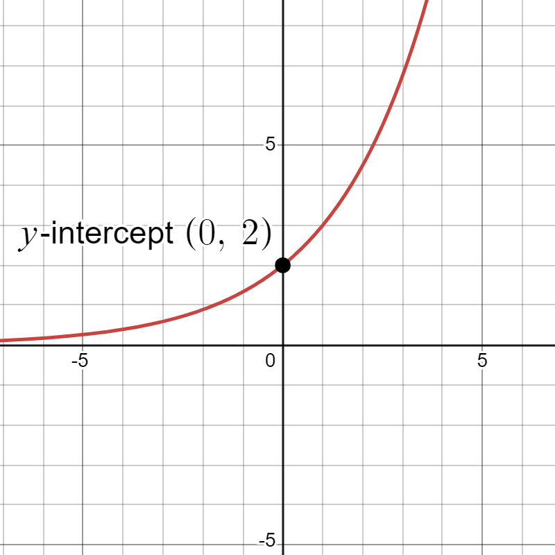
$b > 1$
, we say it models exponential growth. As
$x$
increases, the outputs of the model will increase as well and continue to increase at a much faster rate without bound.
If
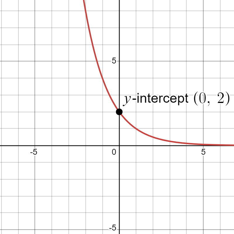
$0 < b < 1$
, the model shows exponential decay. As
$x$
increases, the outputs for the model decrease and continue to decrease, but levels off to the
$x$
-axis (gets close to zero, but will not equal to zero).
When
$x = 0$
the output is
$a$
, so we often call a the initial amount in applications (or the starting amount). We also say
$a$
is also the y-intercept on the graph for the model.
The value b is what we call the growth multiplier. If we increase x by 1, then b is what we multiply the previous output value by to get the new output.

Exponential regression is used to model situations in which growth begins slowly and then accelerates rapidly without bound, or where decay begins rapidly and then slows down to get closer and closer to zero. We use the command “ExpReg” on a graphing utility to fit an exponential model to a set of data points. With Google Sheets or Excel we can use “LOGEST” to find the parameters
$a$
and
$b$
for the exponential model (the methods will be demonstrated in Example 1).

Exponential Regression with Google Sheets Instructions

Enter the data in two rows or two columns in Google Sheets
Find an empty cell with another empty cell to the right. The values for the
$a$
and
$b$
in
$y = a \cdot b^{x}$
will be inserted in those two cells.
Enter the following: =ARRAYFORMULA(LOGEST(data_y_values,data_x_values)), where the data_y_values is the array of y values from the table and data_x_values is the array of x values from the table.
The first value where the function was entered will be
$b$
and the second will be
$a$
for the model
$y = a \cdot b^{x}$
.

Note: At the time of writing this text Google Sheets built in trendline on a scatter plot used a different approach for the values in an exponential model compared to LOGEST. It is recommended you only use the approach as highlighted above in your work as it will match the output from Excel as well as other software. Google Support.

Exponential Regression with Excel Instructions

Office 365

Enter the data in two rows or two columns in Excel
Find an empty cell with another empty cell to the right. The values for the
$a$
and
$b$
in
$y = a \cdot b^{x}$
will be inserted in those two cells.
Enter the following: =LOGEST(data_y_values,data_x_values), where the data_y_values is the array of y values from the table and data_x_values is the array of x values from the table.
The first value where the function was entered will be
$b$
and the second will be
$a$
for the model
$y = a \cdot b^{x}$
.

Office Desktop

Enter the data in two rows or two columns in Excel
Find an empty cell with another empty cell to the right. The values for the
$a$
and
$b$
in
$y = a \cdot b^{x}$
will be inserted in those two cells.
Highlight the two cells for the values and enter the following in the left hand cell: =LOGEST(data_y_values,data_x_values), where the data_y_values is the array of y values from the table and data_x_values is the array of x values from the table. Instead of hitting enter you will need to hold down CTRL+SHIFT+ENTER (CSE) in order to have Excel give an array of values for
$a$
and
$b$
.
The first value where the function was entered will be
$b$
and the second will be
$a$
for the model
$y = a \cdot b^{x}$
.

Example 1

Find the exponential regression model for the data found in the table below:

$x$	1	2	3	4	5	6	7	8	9
$y$	3	5	7	11	19	28	41	67	95

Solution

Before we jump to finding the regression model it is always best to construct a scatter plot for the data to ensure the exponential model seems like a good fit.

Scatter plot y vs x Google Sheet for Exercise

Please be aware that certain images and Google documents may not be properly viewed on mobile devices.

With the data already in a spread sheet (Google Sheets or Excel). Find the values for
$a$
and b for the model.

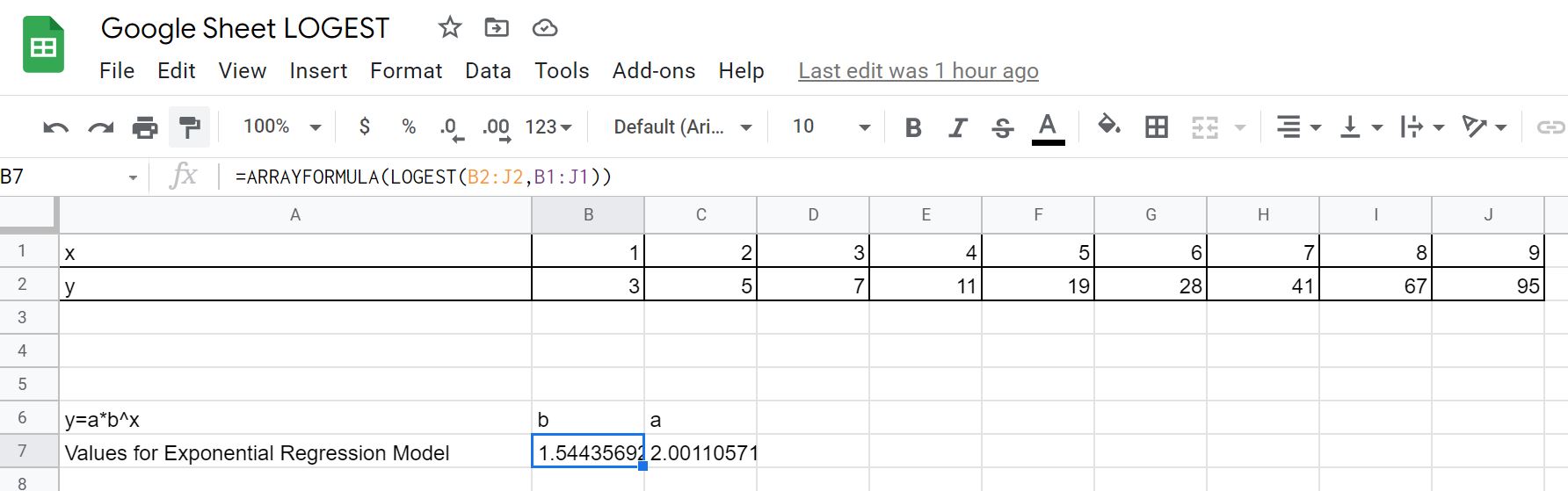
Google Sheets:

A screenshot of the work is shown below where the table values are located in cells B1:J2 with x in the first row and y in the second row. Google Sheet for y vs x

Screenshot of the table of x and y values along with output of the function in B7 =ARRAYFORMULA(LOGEST(B2:J2,B1:J1))

Excel (Office 365):

A screenshot of the work is shown below where the table values are located in cells B1:J2 with x in the first row and y in the second row.

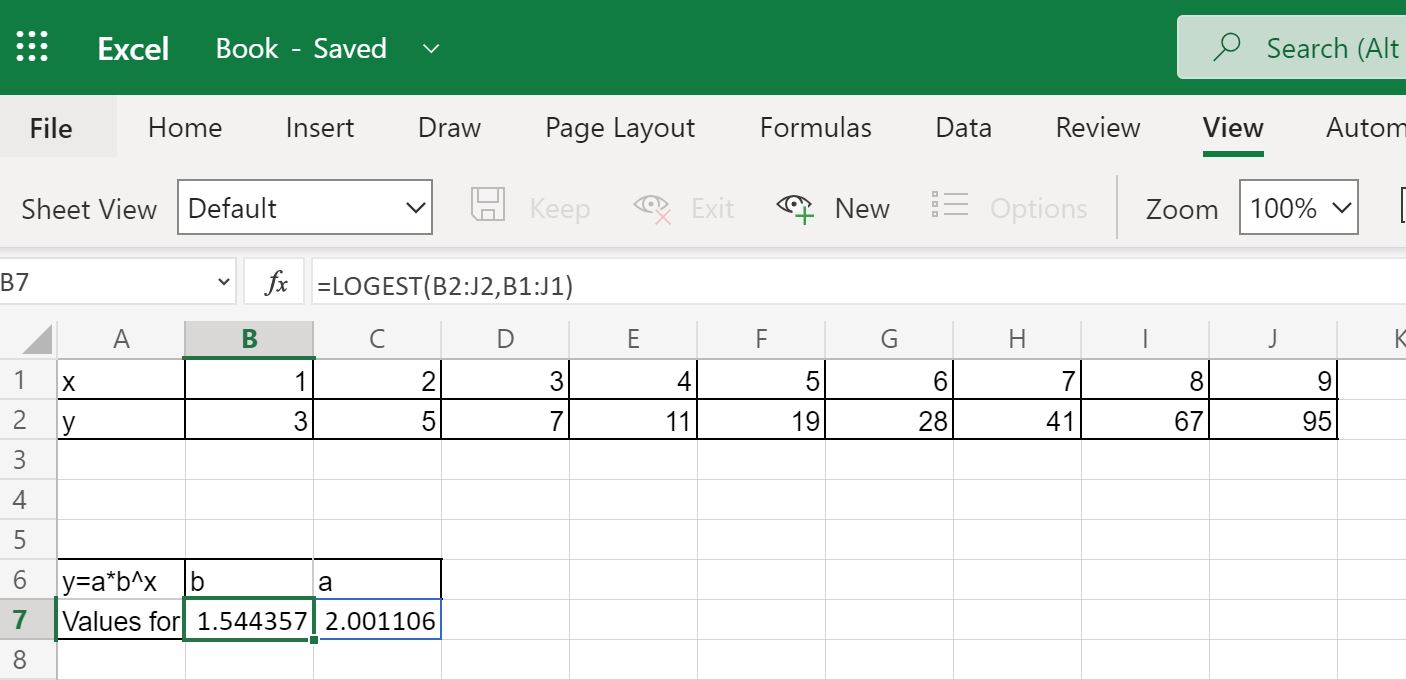
Screenshot of the table of x and y values along with output of the function in B7 =LOGEST(B2:J2,B1:J1)

Final Results:

We see that
$b = 1.5444$
and
$a = 2.0011$
giving us the exponential regression model as
$y = 2.0011 \cdot {(1.5444)}^{x}$

The scatter plot and regression model is given below:

Graph of

y = 2.0011 \cdot {(1.5444)}^{x}

produced on Desmos. Go to Desmos to explore this model.

Like linear regression, finding the exponential regression equation can be done easily with software. There are some cautions though as there are multiple ways to construct the regression line and to match with what we are doing you will need to use the steps described above. If you use something like Desmos you will need to make sure you select the method the log mode method.

Understanding Exponetial Regression in Applications

Remember that exponential regression is used to model situations in which growth begins slowly and then accelerates rapidly without bound, or where decay begins rapidly and then slows down to get closer and closer to zero. Now in some cases that continuation of growth or decay may not always continue, so we must be careful not to extrapolate outside of the given data region as we work with a regression model.

Lets look at some examples on how to find the regression equation and use it to predict outcomes from the model. We will use Google Sheets to do the computations for the regression equation.

Example 2

The following table that relates the total number of confirmed Wuhan Covid cases from January 20 through January 28 in mainland China in 2020. Source: John Hopkins

Total Number of confirmed Wuhan Covid cases in Mainland China
Number of days after January 20, 2020	Total Number of Cases
0	278
1	326
2	547
3	639
4	916
5	2000
6	2700
7	4400
8	5970

Let
$x$
be the number of days after 2020 and
$y$
be the total number of cases. Use exponential regression to fit a model to this data.
What does the model predict for the total number of cases on January 25?
We know it is not wise to extrapolate beyond the original data set, but in some cases we use that extrapolation to help decide on what to currently do (the caveat is that we have to assume the growth will continue at the same rate). Imagine you have the data and it is January 29. You want to give warnings based on the model and show what the predicted values would be in 12 days from now (January 29) if that current growth rate continued. Find the total number of cases predicted based on the model.

Solutions

First thing to do is plot the data to ensure using exponential regression seems reasonable.

Total number of cases vs number of days after January 20, 2020 scatter plot ” Google Sheet for Example 2
Please be aware that certain images and Google documents may not be properly viewed on mobile devices.

Looking at the above scatter plot we do see the increase in number of cases appears to be increasing as well. This is a sign of exponential growth (not just that it is increasing, but the amount of increase is increasing).

Using Google Sheets we get the values for
$a$
and
$b$
in the exponential regression model
$y = a \cdot b^{x}$
. Screenshot below shows what was done:

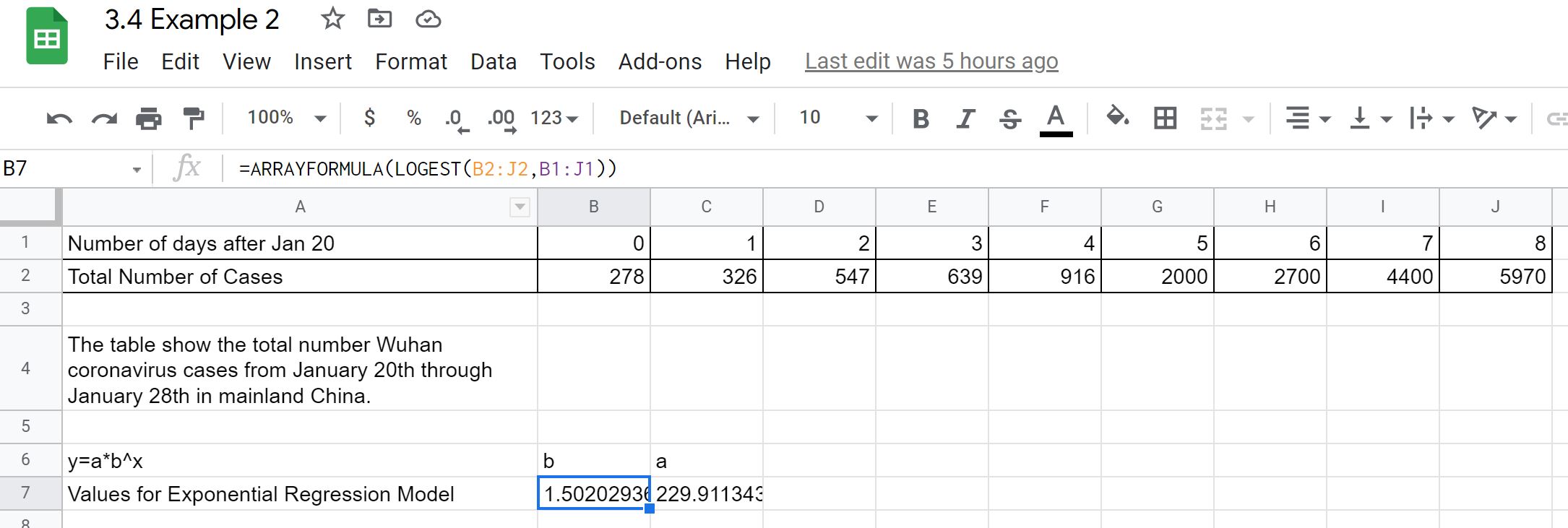
The exonential regression model is
$y = 229.9113 \cdot {(1.502)}^{x}$
.
January 25 would be 5 days after January 20, so we evaluate the model at
$x = 5$
.
$\begin{array}{l} y = 229.9113 \cdot {(1.502)}^{5} \\ y \approx 1758 \end{array}$
The model predicts there would be 1758 total cases on January 25th.
January 29th is already 9 days after January 20 and we want to add on an additional 12 days, so we will evaluate the model at
$x = 9 + 12 = 21$
.
$\begin{array}{l} y = 229.9113 \cdot {(1.502)}^{21} \\ y \approx 1180962 \end{array}$
The model would predict that there would be approximately 1,180,962 total cases. This is a much larger number than what was observed on that day (Feb 10) from the reported data: 42,300. Why the big difference? The government began to take actions on the outbreak prior to January 29 (one of which was a travel ban on Jan 23) as well as many other actions being taken.

Another example below shows how the value of the base can be very large when dealing with very small numbers for the independent variable in the situation.

Example 3

In 2007, a university study was published investigating the crash risk of alcohol impaired driving. Data from 2,871 crashes were used to measure the association of a person’s blood alcohol level (BAC) with the risk of being in an accident. The table below shows results from the study. [Source: Indiana University Center for Studies of Law in Action, 2007] The relative risk is a measure of how many times more likely a person is to crash. So, for example, a person with a BAC of 0.09 is 3.54 times as likely to crash as a person who has not been drinking alcohol.

Relative Risk vs BAC
BAC	0	0.01	0.03	0.05	0.07	0.09	0.11	0.13	0.15	0.17	0.19	0.21
Relative Risk of Crashing	1	1.03	1.06	1.38	2.09	3.54	6.41	12.6	22.1	39.05	65.32	99.78

Let
$x$
represent the BAC level, and let
$y$
represent the corresponding relative risk. Use exponential regression to fit a model to these data.
After 6 drinks, a person weighing 160 pounds will have a BAC of about 0.16. How many times more likely is a person with this weight to crash if they drive after having 6 drinks? Round to the nearest hundredth.

Solutions

Start with constructing the scatter plot to ensure an exponential model is a good fit.

Scatter plot of Relative Risk of Crashing vs BAC Google Sheet for Example 3
Please be aware that certain images and Google documents may not be properly viewed on mobile devices.

From the scatter plot we do see the upward trend in growth that has the look of an exponential model. We find the values for
$a$
and
$b$
for the exponential regression model in Google Sheets and use them to write the equation:

$y = 0.58305 \cdot {(22072021331)}^{x}$

A visual of the scatter plot along with the exponential model is shown below

Graph of
$y = 0.58305 \cdot {(22072021331)}^{x}$
Go to Desmos to explore this model.
Use the model to estimate the risk associated with a BAC of 0.16. Substitute 0.16 for
$x$
in the model and solve for
$y$
.
$\begin{array}{l} y = 0.58305 \cdot {(22072021331)}^{x} \\ y = 0.58305 \cdot {(22072021331)}^{6} \\ y \approx 26.35 \end{array}$
If a 160-pound person drives after having 6 drinks, he or she is about 26.35 times more likely to crash than if driving while sober.

Will it Remain Exponential?

Is it reasonable to assume that an exponential regression model will represent a situation indefinitely?

No. Remember that models are formed by real-world data gathered for regression. It is usually reasonable to make estimates within the interval of original observation (interpolation). However, when a model is used to make predictions, it is important to use reasoning skills to determine whether the model makes sense for inputs far beyond the original observation interval (extrapolation).

Exercises

Find an exponential regression model for the data given in the following table.

$x$ 1 2 3 4 5 6

$y$ 1125 1495 2310 3294 4650 6361

Answer

$y = 776.6824 {(1.4260)}^{x}$
Find an exponential regression model for the data given in the following table.

$x$ 1 2 3 4 5 6

$y$ 555 383 307 210 158 122

Answer

$y = 731.923 {(0.7385)}^{x}$
The table below shows a recent graduate’s credit card balance each month after graduation.

Month 1 2 3 4 5 6 7 8

Debt ($) 620 761.88 899.80 1039.93 1270.63 1589.04 1851.31 2154.92
1. Use exponential regression to fit a model to these data.
2. If spending continues at this rate, what will the graduate’s credit card debt be one year after graduating?
Answer
1. Using Google Sheets the exponential regression model that fits these data is
  $y = 522.88 {(1.1965)}^{x}$
2. If spending continues at this rate, the graduate’s credit card debt will be $4,501.47 after one year.
  $\begin{array}{l} y = 522.88 {(1.1965)}^{x} \\ y = 522.88 {(1.1965)}^{12} \\ y \approx 4501.47 \end{array}$
Data was collected on a particular drugs absorbtion into the body when 1000 mg is given through an IV (see table below).

Time (hours) 0 4 8 12 16 20 24

Debt ($) 1000 580 290 162 93 41 27
1. Construct an exponential regression model for Amount of Drug in body (mg) vs time (hours)
2. Based on that model determine the amount of drugs present after 10 hours.
Answer
1. $y = 1024.57 {(0.8571)}^{x}$
2. Based on that model the amount of drugs (mg) still in the system after 10 hours is 219 mg.
  $\begin{array}{l} y = 1024.57 {(0.8571)}^{x} \\ y = 1024.57 {(0.8571)}^{10} \\ y \approx 219 \end{array}$
It is a safe assumption that box office sales for each week of a movie would follow an exponential model. The table below comes from the first four weeks of Avengers Endgame demostic ticket sales.

Week 1 2 3 4

Ticket Sales (in millions) $474 $187 $81 $40
1. Find an exponential regression model for ticket sales
  $x$
  weeks after opening.
2. What would the model predict for week 6 total ticket sales?
3. Using the model can you find which week the total weekly sales would drop below $1 million dollars?
4. Would there be any reason that the projected sales based on the model would not continue to match up with what actually happened?
Answer
1. $y = 1024.87 {(0.4381)}^{x}$
2. The ticket sales after the 6th week would be approximately 7.25 million dollars.
  $\begin{array}{l} y = 1024.87 {(0.4381)}^{x} \\ y = 1024.87 {(0.4381)}^{6} \\ y \approx 7.25 \end{array}$
3. By trial and error the projected weekly ticket sales drop below 1 million dollars after week 9 (week 9 projected sales are approximately 0.61 million dollars while week 8 projected ticket sales was 1.39 million dollars).
4. Answers will vary. There are various reasons a movies sales may shift away from the model over the passing weeks. One thing that did happen for this movie was getting a boost in ticket sales over the 4th of July weekend. In other cases a movies sales may increase if it started as a limited release and increased the number of theaters it was shown at as the movie became more popular.

License

Icon for the Creative Commons Attribution-NonCommercial-ShareAlike 4.0 International License

5.4 Modeling Exponential Relationships with Regression

3.4

Modeling Exponential Relationships with Regression

Learning Objectives

Exponential Regresion Model

Exponential Model

Exponential Regression with Google Sheets Instructions

Exponential Regression with Excel Instructions

Example 1

Understanding Exponetial Regression in Applications

Example 2

Example 3

Will it Remain Exponential?

Exercises

Answer

Answer

Answer

Answer

Answer

License

Share This Book

Month	1	2	3	4	5	6	7	8
Debt ($)	620	761.88	899.80	1039.93	1270.63	1589.04	1851.31	2154.92

$x$	1	2	3	4	5	6
$y$	1125	1495	2310	3294	4650	6361

$x$	1	2	3	4	5	6
$y$	555	383	307	210	158	122

Time (hours)	0	4	8	12	16	20	24
Debt ($)	1000	580	290	162	93	41	27

Week	1	2	3	4
Ticket Sales (in millions)	$474	$187	$81	$40