5.1 Modeling Linear Relationships with Algebra

5.1: Modeling Linear Relationships with Algebra
Learning Objectives
Upon completion of this section, you should be able to
- Identify elements in a linear model of the form
- Create a linear model with algebra between two quantitative variables
- Graph a linear model
- Solve application problems using a linear model created with algebra
Linear Models
Two variables are in linear relationship if we can describe how they change together by adding or subtracting a fixed constant for each unit increase in one variable. For example the cost for hiring a plumber may start with a $75 fee for coming to your house plus an hourly rate of $60. The two variable here are the total cost for the job and the number of hours needed to complete it. For each one hour increase to complete the job we would see an increase of $60 to the total cost.
What you will work on in this section is how to write an algebraic model to describe that relationship between two variables in applications. We will start with the general equation of a line in slope-intercept form.
Linear Model
A linear model (equation) has the form .
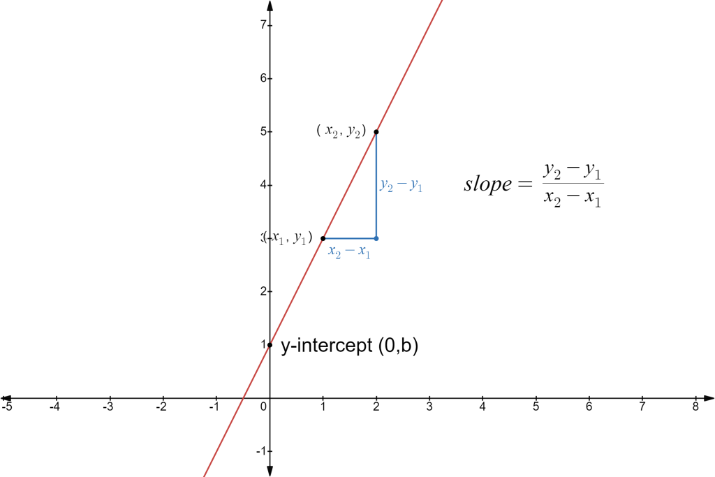
- The is the point at which the graph crosses the . It is indicated by b in the linear model and shown on the graph as the point .
- The slope is a measure of the the line’s steepness, also known as the rate of change. It is represented by m in the linear model . The slope represents the vertical displacement (rise) and horizontal displacement (run) between each successive pair of points. The formula for slope between two points is:
We call this form of a linear equation the slope-intercept form as it gives the information about the slope, m, and y-intercept, b.
Example 1
Which of the following represent a linear model. If it is a linear model identify the slope m and intercept b.
Solution
- This is a linear model. Slope is 10 and the y-intercept is 20.
- This is not a linear model as we are squaring the x term in the equation.
- This is not a linear as the second term in the equation has x in the exponent.
- This is a linear model. We can rewrite it as . The slope is 2 and the y-intercept is 5.
- This is a linear model. We can rewrite it as . The slope is -45 and has a y-intercept of 100.
Before we look at applications lets review how to create a linear model for given sets of points and identify the key elements of slope and intercept.
Example 2
Find a linear model that goes through the points .
Solution
When given two points you start with the slope formula to find m:
Now we were not given the y-intercept directly, so we will first update the linear model with our information about the slope:
Now to find b we can use either of the two given points to put into the equation and solve. We will use in the work below.
Putting our value in for b we get the linear model is:
Try it Now 1
Find the equation of a line that goes through the points .
Hint 1 (click to Show/Hide)
Start with the slope of the line. The slope formula is below. After finding the slope you can use either point given and the slope in the equation to find the y-intercept value b.
Hint 2 (click to Show/Hide)
The slope is:
Answer (click to Show/Hide)
First find the slope of the line:
Next we add the value of the slope to the equation of the line:
Use either point given in the equation to find b, in the work below was used:
The equaiton of the line through is .
Graph a Linear Model by Plotting Points
Linear equations are fundamental in mathematics and have numerous real-world applications. Graphing these equations visually represents their solutions and helps us understand their behavior. One straightforward method to graph a linear equation is by plotting points.
To find points on a graph for any model, we can choose input values (typically represented by x) and evaluate the model at these input values to find the corresponding output values (typically represented by y). The input values and corresponding output values form coordinate pairs (typically represented by (x, y). We then plot the coordinate pairs on a grid.
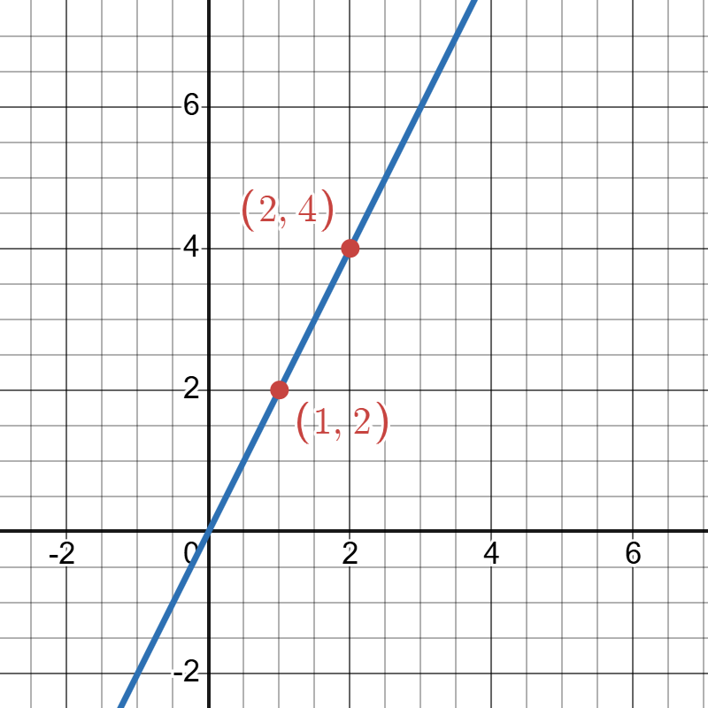
In general, we should evaluate a linear model at a minimum of two inputs in order to find at least two points on the graph. For example, given the model, , we might use the input values 1 and 2. Evaluating the model for an input value of yields an output value of:
This coordinate pair is represented by the point (1, 2). Evaluating the model for an input value of yields an output value of:
This coordinate pair is represented by the point (2, 4). Now that we have two points we first plot the two points and draw a straighline between them as indicated in the graph below.
Click to reveal more information
The image depicts a graph with a grid background showing a Cartesian coordinate system. The x-axis and y-axis intersect at the origin, marked as (0,0). A diagonal blue line passes through two red points, labeled (1,2) and (2,4), indicating the coordinates. The graph grid features lines at regular intervals, with both axes numbered in increments of two. The points are marked with red dots on the line, emphasizing specific locations. The background grid is light gray, and the numbers and labels are written in red text.
Choosing three points is often advisable because if all three points do not fall on the same line, we know we made an error with at least one of the calculations that was done.
Plot by Points Steps
- Choose a minimum of two input values.
- Calculate the corresponding output values.
- Write the input and output values as coordinate pairs.
- Plot the coordinate pairs on a coordinate plane.
- Connect the coordinate pairs with a straight line.
Example 3
Graph the linear model defined by:
Solution
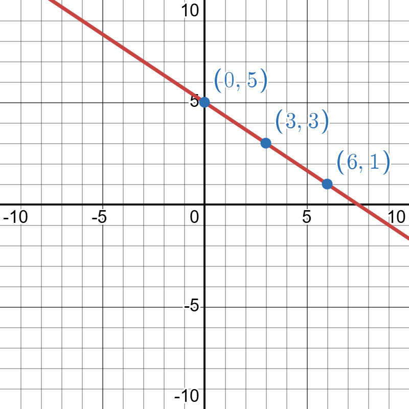
Begin by choosing input values. This linear model includes a fraction with a denominator of 3, so let’s choose multiples of 3 as input values. We will choose 0, 3, and 6.
Evaluate the linear model at each input values, and use the output values to identify coordinate pairs.
Plot the coordinate pairs and draw a line through the points. The graph below is for the model
Click to reveal more information
The image depicts a Cartesian coordinate plane with a red diagonal line extending from the top left to the bottom right. The background is a grid with bold black axes. The x-axis and y-axis are labeled with integer values ranging from -10 to 10. Three blue points intersect the red line at coordinates (0, 5), (3, 3), and (6, 1), each labeled in blue text. The grid is composed of both major and minor grid lines, with minor lines separated by one unit.
The graph has a downward slant when reading left to right over the horizontal axis, which indicates visually a negative slope.
Try it Now 2
Graph the linear model given by
Hint 1 (click to Show/Hide)
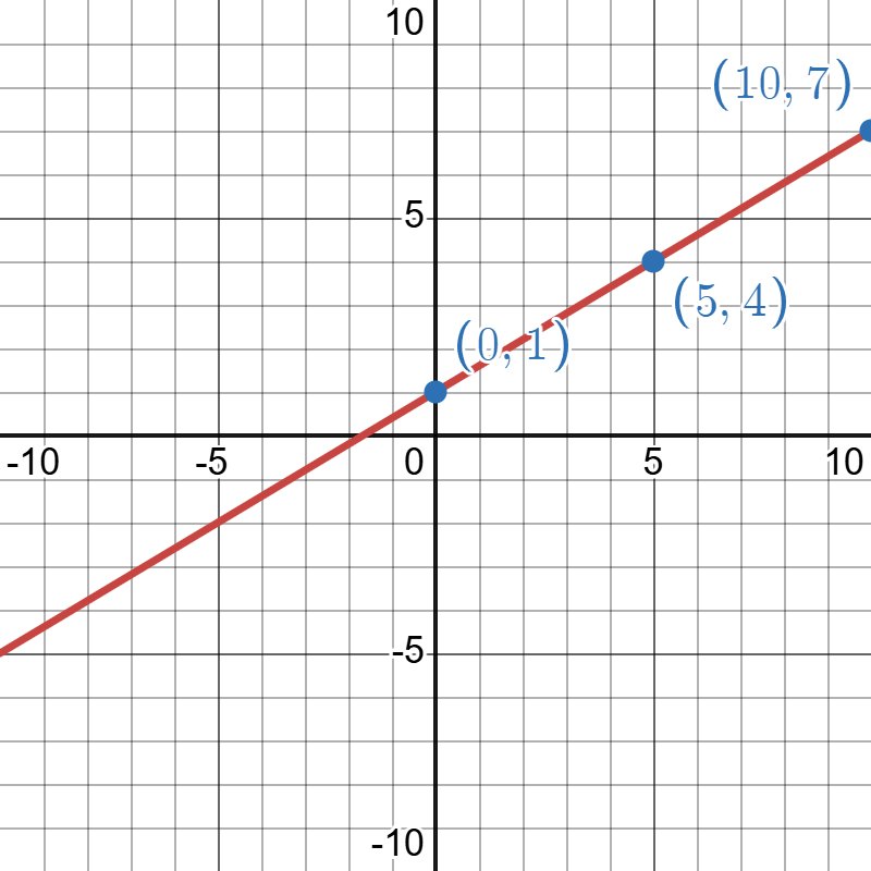
When picking points for the graph it is helpful to identify what may make things easier for you in evaluating the model. Removing the fraction would help. To do this we want to pick values that 5 would divide nicely into as we are multiplying the input value by the fraction . Try using the following:
Answer (click to Show/Hide)
Begin by choosing input values. This model includes a fraction with a denominator of 5, so let’s choose multiples of 5 as input values. We will choose 0, 5, and 10.
Evaluate the function at each input value, and use the output value to identify coordinate pairs.
Plot the coordinate pairs and draw a line through the points as shown below.
Click to reveal more information
The image is a detailed graph on a Cartesian plane with both x and y axes ranging from -10 to 10. The graph displays a red diagonal line with a positive slope, crossing from the bottom left to the top right. Three labeled blue points are marked along the line: (0, 1) at the y-axis, (5, 4) midway along the line to the right, and (10, 7) near the top right. The grid is evenly spaced with black horizontal and vertical lines. Important coordinates are labeled in light blue text near the corresponding points.
Graphing a linear model by using slope and a point
Before we jump into graphing a linear model using the slope and a point let us first review the basic definition given at the beginning of this section.
Linear Model
A linear model (equation) has the form .
- The is the point at which the graph crosses the . It is indicated by b in the linear model and shown on the graph as the point .
- The slope is a measure of the the line’s steepness, also known as the rate of change. It is represented by m in the linear model . The slope represents the vertical displacement (rise) and horizontal displacement (run) between each successive pair of points. The formula for slope between two points is:
We call this form of a linear equation the slope-intercept form as it gives the information about the slope, m, and y-intercept, b.
The y-intercept is a handy point to use when graphing a linear model as it is typically relatively easy to find if it is not given directly. If the linear model is not in the form we can find the y-intercept by setting in the equation and solve for y. The other approach is to solve the linear model for y and then pull the y-intercept directly from that equation.
The other characteristic of the linear model is the slope m, which is a measure of its steepness. Recall that the slope is the rate of change of output to input from the definition. Another way to think about the slope is by dividing the vertical difference, or rise, by the horizontal difference, or run.
If we know the slope and either a point or the y-intercept it is possible to graph the linear model by placing the point on the coordinate system and using the property of the slope to find another point the line goes through. After identifying that next point we can draw the line between the two points or continue to find points on the line using the slope. Choosing at least two points from the slope is often advisable because if all three points do not fall on the same line, we know we made an error.
Graphing a linear model from slope and a point
- Identify a known point on the line. This could be:
- The y-intercept from the equation . This is also found by evaluationg the linear model at .
- Any other given point that satisfies the equation.
- Plot the point on the coordinate plane.
- Use the slope () to determine a second point (if the slope is not in a fractional form you will treat it as a fraction by dividing that number by “1”):
- From the plotted point, move vertically by the numerator of the slope (rise).
- Then move horizontally by the denominator of the slope (run).
- The resulting position gives the second point.
- Sketch the line that passes through the points.
Example 4
Graph the following using information about the slope and the y-intercept:
Solution
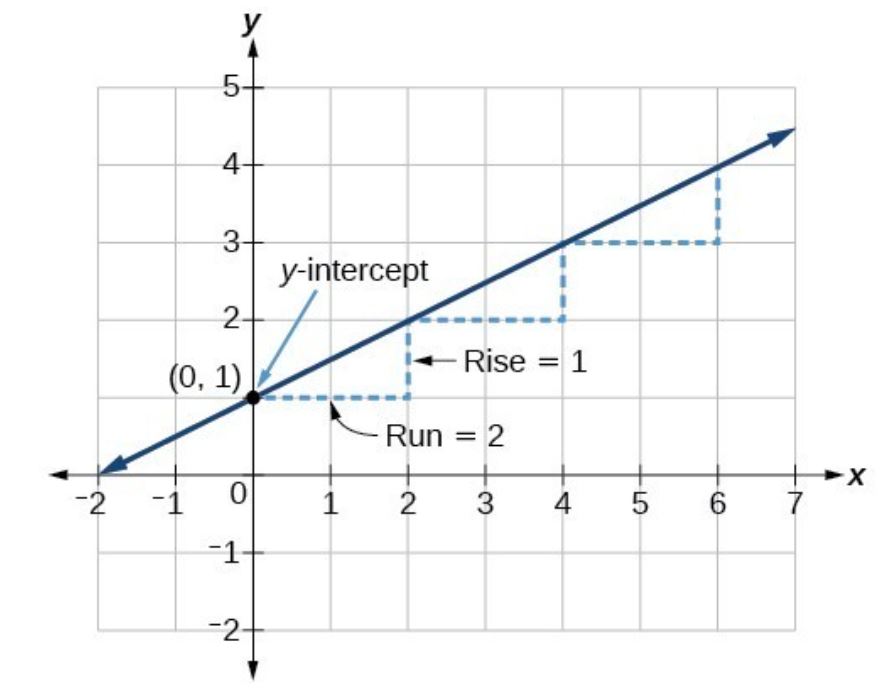
The equation of the line given is already in slope intercept form , so we directly identify both the slope and the y-intercept.
The slope is . Because the slope is positive, we know the graph will slant upward from left to right.
The y-intercept is 1 and is the point on the graph . This is the starting point we can add to the graph shown below.
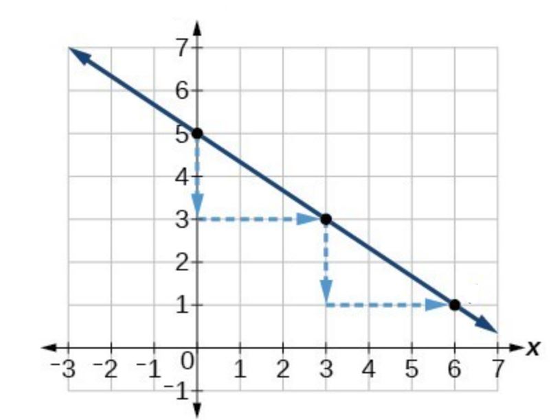
Recall that the slope is the rise over run, . With the slope being , this means that the rise is 1 and the run is 2. So starting from our y-intercept , we can rise 1 and then run 2, or run 2 and then rise 1. We repeat until we have a few points, and then we draw a line through the points as shown below.
Do all linear models have a y-intercept? What about an x-intercept?
The general answer to this is no. Not all linear models have both a y-intercept and an x-intercept. Linear equations can take various forms:
- (slope-intercept form) has both a y-intercept and an x-intercept when and .
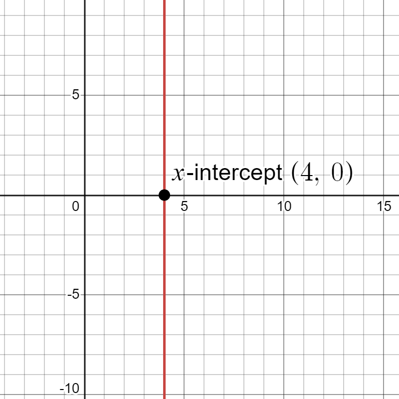
- (vertical line) has an x-intercept at , but no y-intercept (except when where all points are y-intercepts).
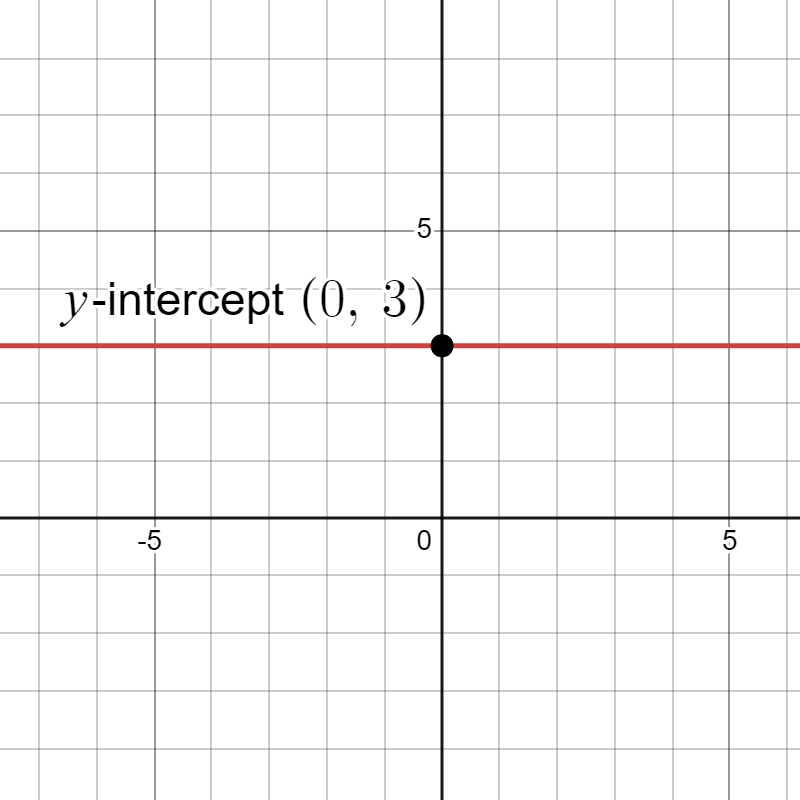
- (horizontal line) has a y-intercept at , but no x-intercept (except when where all points are x-intercepts).
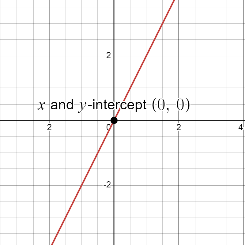
- has both a y-intercept and an x-intercept at the orgin .
While all these are valid linear equations we will focus on linear models of the form , where . These models represent relationships between two variables and typically have both x and y-intercepts.

Try it Now 3
Graph the linear model by using information about the slope and y-intercept:
Hint 1 (click to Show/Hide)
Start by identifying the slope and y-intercept. Recall for the form we know m represents the slope and b the y-intercept.
Hint 2 (click to Show/Hide)
The slope is .
The y-intercept is 5, so we know the point is on the line.
Answer (click to Show/Hide)
The slope is and y-intercept is 5 giving us a point on the graph as .
First thing to note is the slope is negative. This means as we look at the “rise” in the slope it will actually be a decrease (going down). The slope tells us that for each movement in the horizontal direction “run” to the right by 3 units the vertical direction “rise” will decrease (go down) by 2 units.
We can now graph the linear model by first plotting the y-intercept. From the initial value we move down 2 units and to the right 3 units. We can extend the line to the left and right by repeating, and then draw a line through the points.
Solve applications problems involving a linear model
In many real-life situations, we often find that two things (call them variables) are related to each other in a way that can be described by a straight line or linear model. In some situations one variable may explain the value of the other variable in a meaningful way. For example, the number of hours you work would explain the amount you receive on your next paycheck. When we have this type of situation we call that first variable (number of hours) the independent variable and the second (amount on paycheck) the dependent variable.
💡 Tip: Think about cause and effect. The independent variable usually causes or explains a change in the dependent variable.
In most situations the independent variable goes on the x-axis and the dependent variables goes on the y-axis. We often will use different letters than x and y in the model to help relate the variable names to the applications. For example we may use h to represent the hours and w to represent the wages from a paycheck.
Find a linear model in applications: A step-by-step guide
- Identify and Name Variables
- Identify the two main variables being compared
- Assign meaningful letter names to each variable
- Determine Independent and Dependent Variables
- Decide which variable influences the other.
- The influencing variable is the independent (x) variable.
- The affected variable is the dependent (y) variable.
- If there is no direct independent or dependent variable you can randomly assign which to be treated as x and which as y.
- Organize Data as Ordered Pairs
- Write the given information as pairs.
- Use the format: (independent variable, dependent variable)
- Calculate the Slope
- Use the slope formula:
- Find the y-intercept
- Use the slope intercept form for the equation of the line and plug in the value of the slope and pick one of the ordered pairs and enter the values in for x and y. Solve for the unkown value of b to find the y-intercept.
- Write the Linear Model
- Plug in the value for the slope and y-intercept into the linear model in slope intercept form:
Example 5
Research shows that a child’s vocabulary growth is approximately linear between 12 and 18 months of age. (Note: After 18 months, vocabulary tends to grow at a faster rate.) A study tracked a particular child’s vocabulary development with the followng results:
- At 12 months of age: 5 words
- At 18 months of age: 31 words
- Create a linear model for the relationship between the child’s age in months () and their vocabulary size (y).
- Use your model to predict the child’s vocabulary size at 15 months of age.
Solution
First identify the variables. We are given the age of a child and the number of words in the vocabulary. We will use the letter “a” to represent the age of the child and the letter “v” to represent the number of words in the vocabulary.
The age of a child best explains the number of words in the vocabulary. We will treat “a” as the x variable and “v” as the y variable. This gives us our structure for the linear model as:
The information provide in the text gives us two data points in the form .
- At 12 months the child has a vocabulary of 5 words: .
- At 18 months the child has a vocabulary of 31 words: .
Calculate the slope:
Using the information about the slope and the ordered pair we can now find the y-intercept value:
The linear model that relates the age (in months), a, and the number of words in the vocabulary, v, is:
Now to use that model to predict the number of words at 15 months of age we evaluate the model at :
Based on the model the child would be predicted to have a vocabulary of 18 words at the age of 15 months.
What does that y-intercept value from our previous example represent? In this case the y-intercept would not have any meaning in the application as it would represent the number of words in the childs vocabulary at 0 months age. With what was told in the setup of the question a value of 0 for the age would not be okay to use for the linear model.
What about the slope? In the above example we found a linear model that related the childs age in months to the number of words in their vocabulary. The slope was found to be . When the slope was calculated the values used represented:
Putting this together with the values we have the interpretation of 13 words per 3 months. In other words we expect to see a gain of 13 words in the childs vocabulary for every three months of age. The slope is describing the rate of change in the vocabulary for the child with respect to age (in months).
What are the units of slope?
The slope is a ratio of y values to x values, so the units for slope will be the units of y over the units of x:
Example 6
In the Fall of 2019 the PCC tuition for an in-state residents was $84.50 for 1 credit. In Fall of 2020 the tuition for an in-state resident was $87.00 for 1 credit. Construct a linear model for the cost of in-state resident tuition of 1 credit hour assuming the trend is linear and continues in that pattern.
- What does the slope represent in our model?
- What is the predicted tuition in 2024?
- When would the tuition be over $150?
Solution
With the year potentially explaining the tuition cost we have an independent variable of time (the years after 2019) and a dependent variable being the tuition cost. Let t be the time (in years), but we will let represent the year 2019. The dependent variable being tuition cost can be represented by c.
The data that was given to use can be written as a coordinate pair .
- In 2019 the cost for tuition was $84.50, so the corresponding ordered pair is .
- In 2020 the tuition was $87.00 and gives the ordered pair as .
Find the slope based on the data provided:
In this instance we are given the y-intercept as we are using to represent the tuition in 2019 with a value of $84.50. This means the value of b, the y-intercept, is 84.50 for the model.
Putting the slope and intercept into the model we have:
- Our interpretation for the slope is that the tuition will increase by adding $2.50 per year (after 2019) to the total tuition cost. The y-intercept value of 84.50 is the starting tuition amount in 2019.
-
To find the tuition in 2024 we will evaluate the model at as 2024 is fives years after 2019.
-
To find when the tuition is greater than $150 we can set the tuition in the model to 150 and solve for t.
The tuition reaches $150 a little after 26 years. If we use the model for and we see that it is over $150 when or the year 2046.
You may be asking why we wanted the start of the linear model in 2019 to be represented with . The reason for this is to help with reading the model after it is created and having a better understanding of where the tuition started from by looking at the y-intercept value.
When the y-intercept is going to be $84.50; the starting tuition amount in 2019. If we had not picked that starting time as 2019 we would have ended up with a y-intercept that was negative and had no relation to the application for what happens when you enter 0 for the time (year).
Try it Now 4
The population of a small city was in 2012 was 32,500. By 2018 the city has grown to a population of 37,000. If we assume the population is growing with a linear trend, then find a linear model for the city’s population and use the model to answer the following questions:
- What does the slope mean in the model?
- What would the predicted population be in 2021?
- In what year would the population reach 45,000?
Answer (click to Show/Hide)
The two variables are the population and time. The time (year) explains how the population would change, so we will use time as our independent variable and the population as the dependent variable. Like the previous example we will let the time be represented by t, but be the number of years since 2012 (otherwise that y-intercept value would be a value for the population 2000 years ago and would have no meaning to us). The population can be represented with the letter p.
The given information gives us two ordered pairs as .
Calculate the slope:
By our choice for t being the time after 2012 we already know the value of the y-intercept as 32,500. Enter both the slope and y-intercept value to have the linear model: .
Now that the linear model was found answer the given questions.
- The slope represents the rate of change in the population to years. We found the slope to be equal to 750 and means the model is showing the population growing by adding 750 people each year.
- To predict the population in 2021 we need to use as 2021 is 9 years after 2012.
The population in 2021 would be 39,250 based on the model.
- To find the year the population reaches 45,000 we will set and solve for t.
Our model predicts the population will reach 45,000 after 16.67 years from 2012. This would happen sometime in the year 2028.
Exercises
- Identify which are linear models. If it is a linear model state the slope and y-intercept.
Answer (click to Show/Hide)
- Linear: Slope is -1, y-intercept is 10
- Not Linear
- Linear: Slope is , y-intercept is -1
- Not Linear
- Find the equation of a line through the points
Answer (click to Show/Hide)
- Find the equation of a line through the points
Answer (click to Show/Hide)
- Find the equation of a line through
Answer (click to Show/Hide)
- Graph the linear model given by
Answer (click to Show/Hide)
Points picked will vary.
Graph of produced on Desmos. Go to Desmos to explore this model. 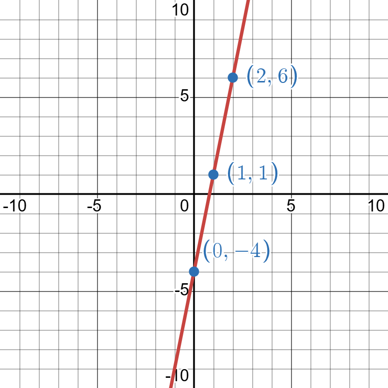
Click to reveal more information
The image is a graph displaying a linear function plotted on a coordinate plane. The graph has a red line passing through several blue points with marked coordinates. The x-axis and y-axis range from -10 to 10, with grid lines at integer intervals. The red line passes through three labeled points: (2, 6) near the top right, (1, 1) in the center right, and (0, -4) below the x-axis. The line has a positive slope. The background consists of a grid providing structure to the graph.
- Graph the linear model given by
Answer (click to Show/Hide)
Points picked will vary.
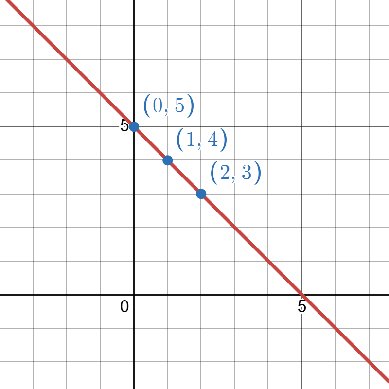
Graph of produced on Desmos. Go to Desmos to explore this model.
Click to reveal more information
The image is a graph with a red diagonal line passing through four quadrants divided by a black x-axis and y-axis. The background consists of a grid with light gray lines. The line descends from the top-left to the bottom-right, intersecting the y-axis at 5. It passes through three blue points marked on the line: (0, 5), (1, 4), and (2, 3). The x-axis and y-axis are labeled with numbers at intervals of 5, with the origin (0, 0) clearly marked. The coordinates are written in blue next to each point.
- Graph the linear model given by
Answer (click to Show/Hide)
Points picked will vary.
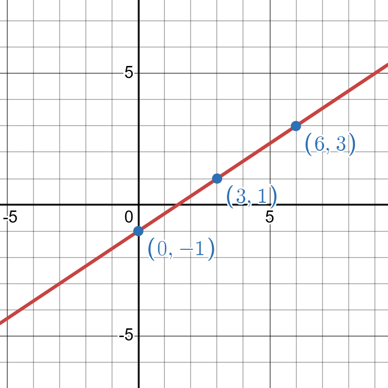
Graph of produced on Desmos. Go to Desmos to explore this model.
Click to reveal more information
The image is a graph plotted on a Cartesian coordinate system with a grid. The x-axis and y-axis intersect at the origin, marked as (0, 0). A red diagonal line extends from the bottom left to the top right, illustrating a linear function. This line passes through three prominent blue points, indicated with coordinates: (0, -1), (3, 1), and (6, 3). Each point is labeled in blue text. The graph is marked with grid lines, and the axes are numbered with intervals of 5.
- The population of beetles is assumed to be growing according to a linear model. The initial population was 30 beetles and after 8 weeks the population reached 62.
- What is a linear model to represent the amount of beetles after t weeks?
- How many beetles would we expect to find after 10 weeks?
- In what week would we expect to see the population reach 150?
Answer (click to Show/Hide)
- 70 beetles after 10 weeks.
- In Week 30.
- The population of a town was 120,000 in 2010. In 2020 the town population was 180,000.
- Write is a linear model to represent the population n years after 2010.
- What does the model predict the population to be in 2025?
- Based on the model when would the population reach 250,000?
Answer (click to Show/Hide)
- 210,000 is the predicted population in 2025.
- Based on the model the population would reach 250,000 during the year 2031.
- A student tutors to help pay for college expenses. If they charge a flat fee of $20 plus $15 an hour, then we can model the total cost of money charges by the following:
Describe what the slope and intercept represent in the model.
Answer (click to Show/Hide)
The slope is 15 in the model. This represents the hourly rate of $15 per hour charged for tutoring.
The y-intercept is 20. This represents the flat fee charged for tutoring.
- A Manufacturer believes there is a linear relationship between the number of widgets, n, they can sell and the price, p, it can charge for the widget. They have historical data that shows they can sell 7,000 widgets at a price of $10 per widget and 1,000 widgets at a price of $25 per widget. Find a linear model that relates the price and number of widgets that can be sold.
Answer (click to Show/Hide)
We will find the linear model in the form:
- An internet provider charges for service based on the model: , where n is the number of GB of data used and C is the monthly charge in dollars. Interpret both the slope and y-intercept for the model in terms of the application.
Answer (click to Show/Hide)
The slope represents the rate of change. In the model there is a slope of 0.15 which would translated as $0.15 per GB of data used.
The y-intercept is an initial value where . In the model the y-intercept is $10 which would mean that there is a flat $10 charge just for service without using any data.
Attributions
This page contains modified content from David Lippman, “Math In Society, 2nd Edition.” Licensed under CC BY-SA 4.0.
This page contains modified content from "College Algebra," Abramson, Jay et al., OpenStax. Licensed under CC BY 4.0.
This page contains content by Robert Foth, Math Faculty, Pima Community College, 2021. Licensed under CC BY 4.0.
